Definition
Kinematic joints are declared by /PROP/KJOINT. Joints are defined by a spring and two local coordinate axes, which belong to connected bodies. Assume that the connected bodies are rigid to ensure the orthogonality of their local axis. However, deformable bodies may also be connected with a joint. If the axis becomes non-orthogonal during deformation, the stability of the joint cannot be ensured.
There are several kinds of kinematic joints available in RADIOSS, which are listed in the following table.
Kinematic Joint Types List
Type No.
|
Joint type
|
dx
|
dy
|
dz
|
θx
|
θy
|
θz
|
1
|
Spherical
|
x
|
x
|
x
|
0
|
0
|
0
|
2
|
Revolute
|
x
|
x
|
x
|
0
|
x
|
x
|
3
|
Cylindrical
|
0
|
x
|
x
|
0
|
x
|
x
|
4
|
Planar
|
x
|
0
|
0
|
0
|
x
|
x
|
5
|
Universal
|
x
|
x
|
x
|
x
|
0
|
0
|
6
|
Translational
|
0
|
x
|
x
|
x
|
x
|
x
|
7
|
Oldham
|
x
|
0
|
0
|
x
|
x
|
x
|
8
|
Rigid
|
x
|
x
|
x
|
x
|
x
|
x
|
9
|
Free
|
0
|
0
|
0
|
0
|
0
|
0
|
x - denotes a blocked degree of freedom
0 - denotes a free (user-defined) degrees of freedom
Joint properties are defined in a local frame computed with respect to two connected coordinate systems. They do not need to be initially coincident. If the initial position of the local coordinate axis coincides at any time, the joint local frames are defined at a mean position. Then the joint local frame will be computed with respect to these rotated axes.
There are a total of six joint degrees of freedom:  X’, Y’, Z’,
  X’, Y’ and Z’. They are computed in the local skew frame.
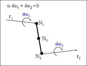
Fig. 4.19: Kinematic joint definition
In each type of joint you distinguish the blocked degrees of freedom and the free degrees of freedom. The blocked degrees of freedom are characterized by a constant stiffness. Selecting a high value with respect to the free degrees of freedom stiffness is recommended. The free degrees of freedom have user-defined characteristics, which can be linear or nonlinear elastic, combined with a sub-critical viscous damping.
The translational and rotational degrees of freedom are defined as follows:
Where, dx1 and dx2 are total displacement of two joint nodes in the local coordinate system.

Where,  and
and  are total relative rotation of two connected body axes, with respect to the local joint coordinate frame.
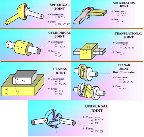
Fig. 4.20: Schematic representation of kinematic joints
Forces and Moments Calculation
The force in direction is computed as:
Linear spring: 
Kt : Translational stiffness (Ktx, Kty, and Ktz)
Ct : Translational viscosity (Ctx, Cty, and Ctz)
Nonlinear spring: 
The moment in direction is computed as:
Linear spring: 
Kr : Rotational stiffness (Krx, Kry, and Krz)
Cr : Rotational viscosity (Crx, Cry, and Crz)
Nonlinear spring: 
The joint length may be equal to 0. It is recommended to use a zero length spring to define a spherical joint or a universal joint. To satisfy the global balance of moments in a general case, correction terms in the rotational degrees of freedom are calculated as follows:
Joints do not have user-defined mass or inertia, so the nodal time step is always used.


