2D Cartesian

2D Cartesian curves or 2D splines consist of two vectors.  Both vectors must be of the same length (or in other words, should have the same number of data points).

2D Parametric

A parametric curve is defined in terms of one free parameter, u. In a 2D Parametric curve C is defined with respect to a coordinate system OXYZ. The coordinates of any arbitrary point on the curve P, as measured in OXYZ, can be represented uniquely in terms of the free parameter u with three functions, f(u), g(u), and h(u), that define the x-, y- and z-coordinates of P. The extent of the curve is governed by the start and end values of u. This is a parametric representation for a curve.  The 2D Parametric curve type available in MotionView is useful in pre-processing such curves.

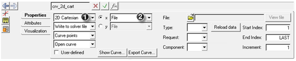
Curve Panel - Properties Tab

2.	From the first drop-down menu , select 2D Cartesian.

3.	From the second drop-down menu , select the curve vector type to define the curve properties.  Each column for the curve can be defined using either of the following vector types:

To know more about how define the curve data using the curve vector types, please refer to the Vector Types topic.

A 2D Curve can also be defined as a User-Defined Curve. Refer to User-Defined topic for additional details.

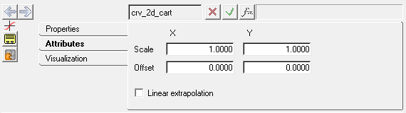
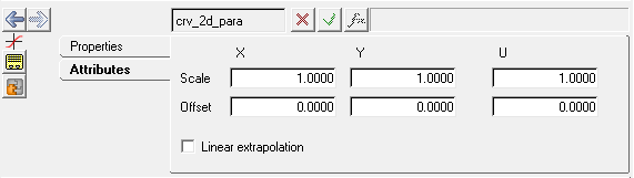
Linear Extrapolation enables the solver to extrapolate the curve linearly when the computed value for the independent variable goes out of the specified bounds.

Syntax:

*Curve(crv_name, "crv_label", 2D,

                             CARTESIAN,

                            [WRITE|NOWRITE],

                            [CONTROL_POINTS|CURVE_POINTS],

                             OPEN|CLOSED])

Example:

*Curve( crv_2d_cart, "2D_Cartesian", 2D, CARTESIAN, WRITE, CURVE_POINTS, OPEN )

The syntax to define the curve data:

*SetCurve(crv_name, Block-X, Block-Y, LIN_EXTRAP )

Block-X and Block-Y can be of the following three types:

FILE: "[path]/filename", datatype, request, component

MATH: expr

VALUE: numpts, v1, v2, v3, ..., vn

Example:

*SetCurve( crv_2d_cart,                FILE, "curve.csv", "Unknown", "Block 1", "column0", FILE, "curve.csv", "Unknown", "Block 1", "column0" )

To understand the complete syntax of the MDL statements mentioned above, please refer to the following MotionView MDL Reference Guide topics: *Curve() and *SetCurve().

MotionSolve writes out the 2D Cartesian curve as Reference_Spline when exported to the MotionSolve XML format.

Syntax:

<Reference_Spline

     id                  = "integer"

   [ label               = "string" ]

   [ linear_extrap       = { "TRUE" | "FALSE" } ]

  {

     usrsub_dll_name     = "valid_path_name"

     usrsub_fnc_name     = "custom_fnc_name" >

   |

     script_name         = valid_path_name

     interpreter         = "PYTHON" | "MATLAB"

     usrsub_fnc_name     = "custom_fnc_name" >

     file_name           = "valid_file_name"

   [ block_name          = "valid_block_name" ]

   | num_x               = "integer"

   [ num_z               = "integer" ] >

    < !-- X       Y for Z1   Y for Z2         Y for ZNUM_Z -->

         x1         y1,1         y1,2       ...        y1,NUM_Z 

         x2         y2,1        y2,2       ...       y2,NUM_Z 

       ...

       XNUM_X        yNUM_X,1      yNUM_X,2     ...    yNUM_X,NUM_Z 

 }

    <!—- Z values -->

      Z1   Z2 ...   ZNUM_Z

</Reference_Spline>

In case of the 2D Cartesian curve, the model statement will be as shown below:

<Reference_Spline

    id                  = "301001"

    label               = "2D_Cartesian"

    num_x               = "9"

    linear_extrap       = "FALSE">

  1.0000000E+00   1.0000000E+00

  2.0000000E+00   2.0000000E+00

  3.0000000E+00   3.0000000E+00

  4.0000000E+00   4.0000000E+00

  5.0000000E+00   5.0000000E+00

  6.0000000E+00   6.0000000E+00

  7.0000000E+00   7.0000000E+00

  8.0000000E+00   8.0000000E+00

  9.0000000E+00   9.0000000E+00

 </Reference_Spline>

To understand the complete syntax of the Reference_Spline XML model statement, please refer to the MotionSolve Reference Guide topic for Reference_Spline.

In MotionView, Tcl can be used to add any MDL entities to the model.  There are two Tcl commands that can be used to add an entity:

InterpretEntity

InterpretSet

The InterpretEntity command is used to add entities to the model and the InterpretSet command is used to set the entity properties.  To understand the complete usage and syntax of these commands, please refer to the InterpretEntity and InterpretSet topics located within the HyperWorks Desktop Reference Guide.

Note - When using the InterpretEntity and InterpretSet commands, it is important to also use the Evaluate command in order for the changes to take effect immediately.

To learn how to create a complete model using Tcl commands, please refer to tutorial MV-1040: Model Building Using Tcl.

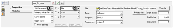
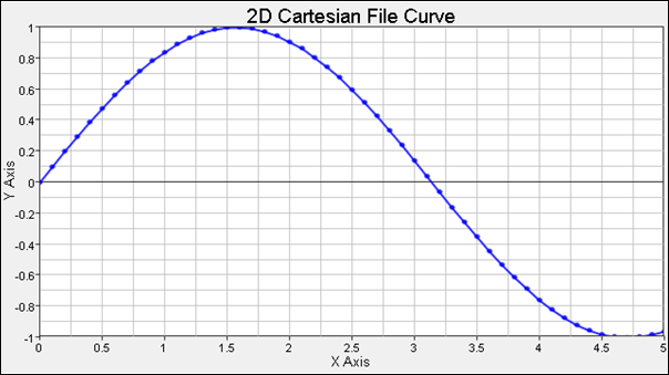
In the case of a Parametric curve, a parameter U will be introduced more arbitrarily, mainly as a tool for describing the curve. One often uses the language of a point "moving" along the curve even in more abstract situations where the curve does not have a mechanical interpretation.

An example use case for using 2D parametric curves is discussed below. The data of the u parameter of the curve is available in a File vector type.  The X and Y vectors of the 2D Parametric curve are derived from the File based U vector.

The example curve could be represented like this:

The values for the X and Y are computed using the Math expressions, by taking the u parameter as the reference values.

Curve Panel - Properties Tab

2.	From the first drop-down menu , select 2D Parametric.

3.	From the second drop-down menu , select the curve vector type to define the curve properties.  Each column for the curve can be defined using either of the following vector types:

To know more about how define the curve data using the curve vector types, please refer to the Vector Types topic.

Syntax:

*Curve(crv_name, "crv_label", 2D,

                             PARAMETRIC,

                            [WRITE|NOWRITE],

                            [CONTROL_POINTS|CURVE_POINTS],

                            OPEN|CLOSED])

Example:

*Curve( crv_2d_para, "2D_Parametric", 2D, PARAMETRIC, WRITE, CURVE_POINTS, OPEN )

The syntax to define the curve data:

*SetCurve(crv_name, Block-U, Block-X, Block-Y, LIN_EXTRAP )

Block-X and Block-Y can be of the following three types:

FILE: "[path]/filename", datatype, request, component

MATH: expr

VALUE: numpts, v1, v2, v3, ..., vn

Example:

*SetCurve( crv_2d_para, FILE, "curve.csv", "Unknown", "Block 1", "column0", MATH, cos(crv_2d_para.u), MATH, sin(crv_2d_para.u) )

To understand the complete syntax of the MDL statements mentioned above, please refer to the following MotionView MDL Reference Guide topics: *Curve() and *SetCurve().

MotionSolve writes out the 2D Cartesian curve as Reference_Spline when exported to the MotionSolve XML format.  The syntax for the 2D Parametric curve is same as the 2D Cartesian curve.  While getting exported to XML, MotionSolve writes out the values for X and Y by taking the U parameter as the reference value.  The extent of the curve is governed by the number of U points (that is, the start and end points).

Syntax:

<Reference_Spline

     id                  = "integer"

   [ label               = "string" ]

   [ linear_extrap       = { "TRUE" | "FALSE" } ]

  {

     usrsub_dll_name     = "valid_path_name"

     usrsub_fnc_name     = "custom_fnc_name" >

   |

     script_name         = valid_path_name

     interpreter         = "PYTHON" | "MATLAB"

     usrsub_fnc_name     = "custom_fnc_name" >

     file_name           = "valid_file_name"

   [ block_name          = "valid_block_name" ]

   | num_x               = "integer"

   [ num_z               = "integer" ] >

    < !-- X       Y for Z1   Y for Z2         Y for ZNUM_Z -->

         x1         y1,1         y1,2       ...        y1,NUM_Z

         x2         y2,1        y2,2       ...       y2,NUM_Z

       ...

       XNUM_X        yNUM_X,1      yNUM_X,2     ...    yNUM_X,NUM_Z 

 }

    <!—- Z values -->

      Z1   Z2 ...   ZNUM_Z

</Reference_Spline>

To understand the complete syntax of the Reference_Spline XML model statement, please refer to the MotionSolve Reference Guide topic for Reference_Spline.

In MotionView, Tcl can be used to add any MDL entities to the model.  There are two Tcl commands that can be used to add an entity:

InterpretEntity

InterpretSet

The InterpretEntity command is used to add entities to the model and the InterpretSet command is used to set the entity properties.  To understand the complete usage and syntax of these commands, please refer to the InterpretEntity and InterpretSet topics located within the HyperWorks Desktop Reference Guide.

Note - When using the InterpretEntity and InterpretSet commands, it is important to also use the Evaluate command in order for the changes to take effect immediately.

To learn how to create a complete model using Tcl commands, please refer to tutorial MV-1040: Model Building Using Tcl.

*BeginMDL( the_model, "Model", "12.0.110.20" )

 *StandardInclude(FILE)

 *SetCurrentSolverMode(MotionSolve)

 *Point( p_a, "Point A" )

 *Body( b_a, "Body A", p_a, , , ,  )

 *Set( b_a.usecm, true )

 *ActionOnlyForce( frc_cart_crv, "Force_Cartesian_Curve", TRANS, b_a, p_a, Global_Frame )

 *ActionOnlyForce( frc_para_crv, "Force_Parametric_Curve", TRANS, b_a, p_a, Global_Frame )

// Example for 2D Cartesian Curve

 *Curve( crv_2d_cart, "2D_Cartesian", 2D, CARTESIAN, WRITE, CURVE_POINTS, OPEN )

 *SetCurve( crv_2d_cart,                FILE, "D:/Documents/curve.csv", "Unknown", "Block 1", "column0", FILE, "D:/Documents/curve.csv", "Unknown", "Block 1", "column0" )

// Example for a 2D Parametric Curve

 *Curve( crv_2d_para, "2D_Parametric", 2D, PARAMETRIC, WRITE, CURVE_POINTS, OPEN )

 *SetCurve( crv_2d_para,                FILE, "D:/Documents/curve.csv", "Unknown", "Block 1", "column0", MATH, cos(crv_2d_para.u), MATH, sin(crv_2d_para.u) )

 *SetForce( frc_cart_crv,               CRV, crv_2d_cart, , , LIN, , LIN )

 *SetForce( frc_para_crv,               CRV, crv_2d_para, , , LIN, , LIN )

 *SetActiveAnalysis( NONE )

*EndMDL()