Grid Participation - Display Options Dialog

The Display Options dialog allows you to customize the response plot using the following options:

nvh_grid_part_display_options_ld_stdy_tab_hv

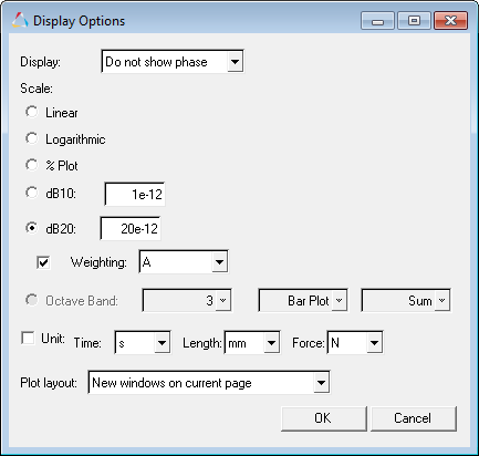
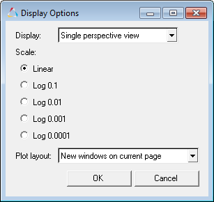
Load tab and Study tab - Display Options dialog

Display tab - Display Options dialog

Display

The following options are available from the Display drop-down menu:

	Do not show phase	Hides the phase values on the plot.
	Show phase	Displays the phase values on the plot.
	Single perspective view (available for the Display Tab only)	Displays a contour plot using only the isometric perspective.
	Multiple perspective view (available for the Display Tab only)	Displays multiple contour plots using the isometric, top, and bottom perspectives.

Scale

Displays the scale types available.

Be sure to review the various scaling types in order to determine which type gives you the best spatial location of the contributions.

For example, the Linear scale type is not very useful when looking at a Structure grid participation (the very localized red contributions displayed on the model) because it makes it extremely difficult to see the contributions. In many instances this contribution can be concentrated at one single point, and if there is only one grid contributing, then you essentially will not be seeing a very clear picture of where it is contributing. If that is the case, you will need to use another kind of scaling in order to make the area larger so that you will actually see a patch of the surface that contributes. You therefore want to find a scaling type which localizes the contribution without making the area too small to easily locate.

Note	The Log extreme scaling versions are available for review (essentially everything on the model is displayed in red or blue); however these results are usually not very useful because they show that everything is equally effective in fixing the problem.

Linear

Plots the linear values.

Logarithmic

Plots the values in logarithmic scale. With this scale, data points are spread out more, which makes it easier to view.

Log 0.1
(available for the
Display Tab only)

Logarithmic scale with a reference value of 0.1.

Log 0.01
(available for the
Display Tab only)

Logarithmic scale with a reference value of 0.01.

Log 0.001
(available for the
Display Tab only)

Logarithmic scale with a reference value of 0.001.

Log 0.0001
(available for the
Display Tab only)

Logarithmic scale with a reference value of 0.0001.

% Plot

Plots the contribution of the selected modes as a percentage of the total response. Percentage plot is a good option to use when comparing contributors versus the total response.

dB10

10 logarithmic of the participation value over the reference value.

dB20

20 logarithmic of the participation value over the reference value. For acoustic responses, the reference pressure is 20E-12 MPa.

Weighting

A – A-weighting used to define equal loudness sound pressure levels.

B – B-weighting used to define equal loudness sound pressure levels.

C – C-weighting used to define equal loudness sound pressure levels.

U – U-weighting used to define equal loudness sound pressure levels.

Unit

Activate the Unit check box and make selections from the following drop-down menus:

•	Time (s, ms)

•	Length (mm, m, ft, km, mile, inch)

•	Force (N, KN, lbf)

Plot Layout

Select how the plot window will appear.

	New windows on current page	Plot is placed into a new window on the current page.
	Active window	Plot is placed into the active window.
	New windows on new page	Plot is placed into a new window on a new page.