Title
VPG with flexible and rigid bodies
|
|
Number
14.2
|
Brief Description
After applying gravity, a truck runs on a horizontal plane and passes over a bump. The major part of the truck is described using a flexible body.
|
Keywords
| • | Eigen and static analysis |
|
RADIOSS Options
| • | Eigen modes computation (/EIG) |
| • | Flexible body input file (/FXINP) |
|
Input File
VPG_Rigid_body: <install_directory>/demos/hwsolvers/radioss/14_Truck_with_FXB/VPG_Rigid_body/TRUCK*
VPG_Flexible_body: <install_directory>/demos/hwsolvers/radioss/14_Truck_with_FXB/VPG_Flexible_body/Model_EIG/TRUCK_EIG_*
<install_directory>/demos/hwsolvers/radioss/14_Truck_with_FXB/VPG_Flexible_body/Model_FXB/TRUCK_FXB_*
|
Technical / Theoretical Level
Advanced
|
Overview
Aim of the Problem
The purpose of this example is to perform an Eigen analysis on a complete truck model with the purpose of creating a flexible body which will be used to model the truck’s main part, excluding transmission (wheels, left-springs, differential, shaft, brakes and axles). In order to appreciate the quality of the modeling, the results will be compared with those obtained using two other models: one without a flexible body (previous analysis) and the other substituting the flexible body with a rigid body.
The study deals with:
| • | an Eigen analysis to create a file containing the dynamic response of the structure |
| • | a quasi-static analysis (explicit pre-loading by gravity) |
| • | an explicit dynamic analysis with a global flexible body |
| • | an explicit dynamic analysis with a global rigid body |
Analysis, Assumptions and Modeling Description
Modeling Methodology
The original model and two alternative models are compared:
1 complete model
|
1 model including a
global flexible body
|
1 model including a
global rigid body
|
In the previous section where a complete finite element model is used, it is noted that the stress and strain levels are low for most parts of the global model. Thus, the CPU time can be considerably reduced if the elements working in the linear elastic field are replaced with a flexible body. The purpose of this example is to provide an overall view of using flexible bodies in RADIOSS.
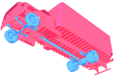
The top part of the truck, where no damage and no plastic strain occurs, is first successively modeled with a rigid body (non-deformable) and then with a flexible body (deformable), as shown in Fig 20.
Parts of the truck covered by rigid or flexible body is shown in the following diagram:
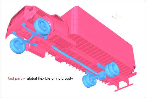
Fig 20: Top part of truck included in a flexible/rigid body depending on the model.
RADIOSS Options Used
Eigen and Static Modes Computation – Flexible Body Creation
A flexible body is similar to a rigid body where displacement is computed on nodes corresponding to vibration modes. The input file for a flexible body uses the RADIOSS Eigen modes and static modes computation. Modes can derive from experimental analysis, as well as from vibratory software.
The total displacement field for every point of a flexible body is obtained by displacing the local frame defining the rigid body modes and from an additional local displacement field corresponding to the body’s small vibrations.
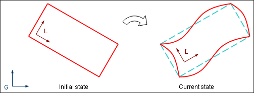
Fig 21: A flexible body is deformable according to its Eigen modes (from vibratory analysis).
A preliminary study with RADIOSS extracts Eigen or static modes for creating the flexible body input file used in a second run. This computation phase requires the /EIG and /FXINP options.
The /EIG option is set up in the Starter input file and defines the part to be included in the flexible body, as well as the type and number of modes to be computed.
In this example, the main data is:
| • | Maximum Eigen frequency = no |
| • | Minimum Eigen frequency = 13 Hz |
| • | Number of Eigen modes per block = 10 |
Two types of modes can be obtained:
Eigen modes (or dynamic modes) are computed for the entire structure without any specific boundary condition. The equation solved is:
Ku =  Mu
Mu
In this approach, rigid body modes in the structure are possible and give null Eigen frequencies.
If Kur = 0, K is not singular and ur  0, therefore, Mur = 0 and = 0
In addition, static modes can be computed if boundary conditions are added to a node group in the flexible body frontier. They correspond to the static response of the structure. All degrees of freedom in the set of interface nodes concerned by the additional boundary conditions are fixed and one static mode is computed for each constrained degree of freedom. The equation solved is:
Ku = F
Static modes are displayed with null frequencies in animations.
Rigid modes are not permitted and generate null pivots during inversion of the stiffness matrix.
It should be noted that modes computation requires the implicit options in the Engine file (/IMPL/LINEAR and /IMPL/SOLVER/1).
| • | Eigen frequencies are provided in the Engine output file. One animation exists per computed mode. |
| • | The /FXINP option is used in the Engine file for creating a flexible body input file .fxb. The flexible body has the same support as that defined in /EIG. You should enter: |
| - | Identification number of the Eigen mode or static mode problem defined in /EIG; |
| - | The critical structural damping coefficient used for computing the Rayleigh damping coefficient to be introduced in the flexible body (it is recommended to use default value 0.03); |
| - | Type of flexible body (1 = free flexible body, 2 = fixed flexible body). |
| • | The flexible body input file can be used in a second run using /FXBODY in the Starter Input file to generate a flexible body. The flexible body input file name ending in .fxb for the RADIOSS format and master node coordinates are required (possible coordinates are given at the top of the .fxb file). |
|
Eigen Analysis (writing FXB input file)
|
Run using Flexible Body
|
FXB domain can contain
|
R Rigid bodies + master nodes.
R Boundary conditions.
|
R Master nodes of rigid bodies.
R Master node of the flexible body.
R Interfaces.
|
FXB domain must not contain
|
T Free parts.
T Slave nodes on the flexible body frontier.
T Rigid body overlapping on flexible body and the rest of structure.
T Truss elements.
T Void material.
T Monitored volumes.
|
T Rigid bodies (slave nodes).
T Slave nodes on the flexible body frontier.
T Rigid body overlapping on flexible body and the rest of structure.
|
Options incompatible with the implicit solver must be avoided.
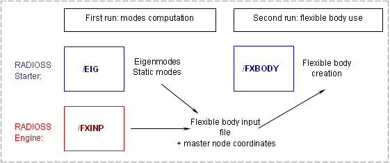
Fig 22: Flexible body creation from RADIOSS options.
The inputs files used with the specific options are:
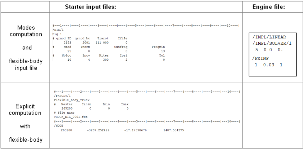
For the truck model, the global flexible body includes 14344 nodes, 120 of which are the master nodes of the inside rigid bodies. Thus, the flexible body takes into account constraints of the rigid bodies.
Eigen Run
In addition, you can define nine interface nodes linking the flexible body and the rest of the truck with the translation fixed along the X-, Y- and Z-axis. Thus, 27 static modes will be computed.
Only the translation degrees are retained in order to minimize the input file size of the flexible body, given that preliminary studies have shown that additional static modes computed by fixing rotational degrees have not substantially improved flexible body behavior.
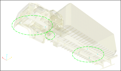
Fig 23: Nine interface nodes with blocked translations for computing static modes.
A static mode is computed for each fixed degree of freedom, in addition to the Eigen modes. Thus, the number of modes is equal to the number of Eigen modes, plus the number of blocked degrees of freedom.
Flexible Body Run
The rigid bodies and tied interfaces included in the flexible body domain should be removed for the second run. Those kinematic conditions are only considered in Eigen modes computation.
The coordinates of the center of mass (possible master node) indicated in the flexible body input file are:
X: 3.267252E+03 Y: -1.71759E+01 Z: 1.407584E+03 (node 265200)
The master node should be included in the nodes groups for gravity loading and initial velocity. It should be defined in the Starter file (/NODE).
Connections between the parts covered by the flexible body and other parts of the model are modeled with beams and the rigid body, as shown in Fig 24. Connection is set at the beam extremity.
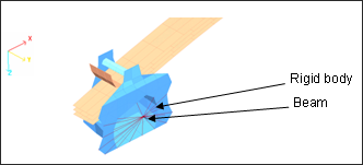
Fig 24: Example of the connection point for flexible body.
Simulation Results and Conclusions
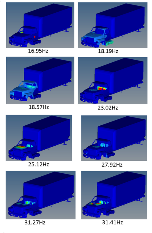
Fig 25: Characteristic Eigen modes (arbitrary displacement).
Comparison of Animation Results
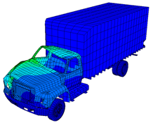
Deformed configurations are compared with global bodies according to the modeling used:
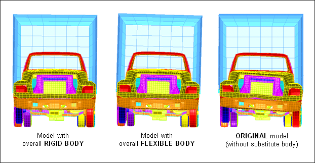
Fig 26: Face view of the different models’ behavior during bump passage (displayed with multi-models option)
Animation Results
| • | Animations multi models: cab deformation face view |
| • | Animation flexible body model: cab deformation |
| • | Animation original model: cab deformation |
Conclusion
This example introduced a method for creating and employing a flexible body using an Eigen analysis performed by RADIOSS. The number of retained modes and the frequency range set for the Eigen analysis are according to the parameters which influenced the results.
Simulation using the flexible body provided accurate distribution of deformations in the model, compared with the modeling not having a substitute body. However, the amplitudes obtained are very low. The flexible body behavior could be enhanced by improving connections between the flexible body and the rest of the structure to ensure transmission of the shock wave up to the flexible body.
The flexible body input file required the IMPLICIT module for the Eigen modes computation.


