Title
VPG with a complete finite element model
|
|
Number
14.1
|
Brief Description
After applying gravity, a truck runs on a horizontal plane and passes over a bump.
|
Keywords
| • | Shell, brick, beam, beam type spring, and monitored volume (perfect gas) |
| • | Quasi-static load treatment and kinetic relaxation |
| • | Type 7 and 2 interfaces, self-impacting, and rigid wall (infinite plane and cylinder) |
|
RADIOSS Options
| • | Boundary conditions (/BCS) |
|
Input File
VPG_complete_model: <install_directory>/demos/hwsolvers/radioss/14_Truck_with_FXB/VPG_complete_model/TRUCK*
|
Technical / Theoretical Level
Advanced
|
Overview
Physical Problem Description
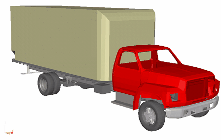
The truck model is placed on the ground under the gravity field until static equilibrium is obtained. Then, under the impulse of 15.6 m/s (56 km/h) initial speed, the truck runs in a straight line and passes over a speed bump. The shock is expected to cause major deformation in some highly solicited parts.
Units: mm, s, ton, N, MPa.
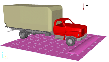
Fig 1: Problem studied.
In order to simplify modeling, most of the parts undergo the linear elastic material law (/MAT/LAW1).
| • | Young’s modulus: 205000 MPa |
The elasto-plastic Johnson-Cook model (/MAT/LAW2) mainly describes the joint and strengthening elements, such as the beams and spring.
| • | Young’s modulus: 205000 MPa |
| • | Hardening parameter: 480 MPa |
The truck represents a simplified model having the essential parts. The weight of the truck is approximately 8 tons.
Analysis, Assumptions and Modeling Description
Modeling Methodology
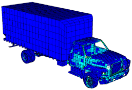
Finite Element mesh:
The truck model is meshed with 21430 elements - 148356 degree of freedom, as follows:
Details of the elements used are provided in Table 1 below:
Table 1: Composition of the EF mesh.
|
Number
|
Node
|
24726
|
4-node shell
|
18471
|
3-node shell
|
1638
|
Brick
|
1148
|
Beam
|
47
|
Spring
|
126
|
Part
|
159
|
The improved Belytschko hourglass formulation (type 4 hourglass, Ishell =4) is used for shell elements in the explicit computation. The Eigen analysis requires fully-integrated elements since the computation mode needs an implicit option. Compatible element formulations are set by default.
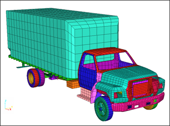
Fig 3: Overall mesh of truck.
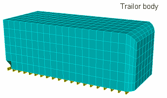
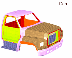
The main parts of the model are shown in the table below:
Fig 4: Definition of the part.
Monitored Volumes / Perfect Gas
Monitored volumes are used to model the pressure in the tires. They are defined with one or more shell property sets and the surface must be closed. The monitored volume used is the perfect gas type.
The main properties for this type are:
| • | External pressure: 0.1 MPa |
| • | Initial internal pressure: 0.3 MPa |
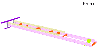
All other properties are set to the default values. The parts modeled with the monitored volumes are highlighted in Fig 5:
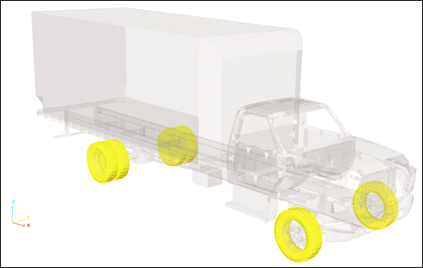
Fig 5: Visualizing the monitored volumes (yellow parts).
Connections Between Parts
In order to assemble the parts, four link types are used in the model:
| • | Rigid body (kinematic condition) |
| • | Tied interface type 2 (kinematic condition) |
The beam type spring elements are useful for modeling the welding points. The modeling techniques are described in the RADIOSS User's Guide.
In this example the beam type spring properties are:
| • | Young’s modulus: 210000 MPa |
Force and moment are read from the input curves:
Table 2: Input force versus displacement curve.
Displacement
|
-1
|
0
|
1
|
Fx, Fy, Fz
|
-105
|
0
|
105
|
Table 3: Input moment versus rotation curve.
Rotation
|
-1
|
0
|
1
|
Mx, My, Mz
|
-106
|
0
|
106
|
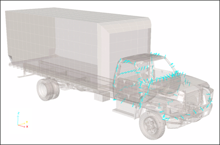
Fig 6: Beam type springs (13) used in the model.
The type 2 tied interface rigidly connects a set of slave nodes to a master surface. The kinematic constraint is set on the slave nodes which remain in the same position on their master segments. This interface is a kinematic condition. The Spotflag spotweld formulation is set to zero in order to connect two meshes without coincident nodes. The master surface should be the coarser mesh.
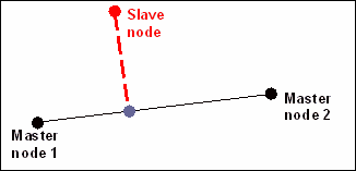
Fig 7: Tied interface (type 2).
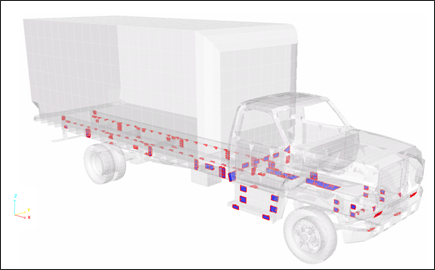
Fig 8: Tied interfaces (type 2) used in model
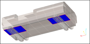
Fig 9: Example of the tied interface modeling connections between the fuel tank and its support
Rigid bodies are created to join two or more parts together. For these rigid bodies no added mass is required and the master node can be located anywhere.
Slave nodes may not accept the other kinematic conditions (such as tied interface).
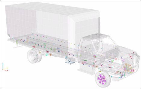
Fig 10: Visualization of rigid bodies in model.
A spherical inertia must be used for the rigid bodies having only two slave nodes for ensuring the stability of the connected elements (set Ispher = 1). Thus, inertia is spherical and not computed from data.
Contact Modeling – Self-impacting
Taking into account self-impacting parts, a type 7 self-impacting interface must be used. The Block Format definition of this interface is to define master surface (/SURF/PART), then define slave nodes as all nodes on this surface (/GRNOD/SURF).
Gap is equal to 0.5 mm.
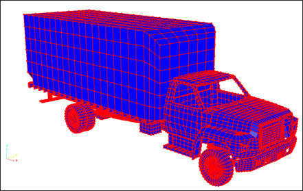
Fig 11: Type 7 interface – self-impacting (slave side in red and master side in blue).
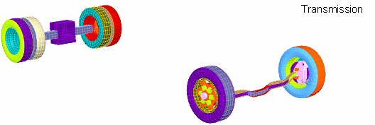
Wheel Rotation Modeling
Wheels are linked to a frame using an axle attached to the brake systems. A beam element (in red in the opposite figure) models the axle causing released rotations at the node linked to the wheel rim.
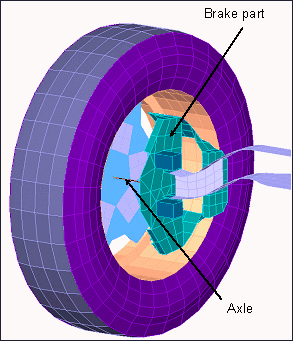
Fig 12: Wheel model (without brake disk)
RADIOSS Options Used
Two types of rigid walls are set up:
| • | A fixed infinite plane (ground); |
| • | A fixed infinite cylinder having a diameter, D = 1500 mm (bump). |
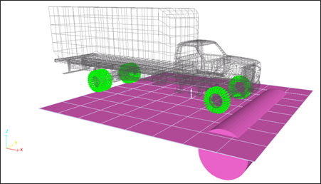
Fig 13: Infinite plane and cylindrical wall for modeling the ground and bump (slave nodes displayed in green).
The cylindrical wall is defined by point M (500, 0, -600), M1 (500, 100, -600) and the diameter.
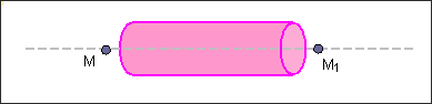
Fig 14: Cylindrical wall definition.
Both rigid walls are tied to allow the wheels to turn. The tire parts define the slave nodes for the infinite plane (contact of ground and tires) and only the nodes of the front right tire are set as slave for the speed bump in order to model a local bump. The obstacle is not infinite.
A kinematic condition is applied on each impacted slave node. Therefore, a slave node cannot have another kinematic condition; unless such condition is applied in an orthogonal direction. In such a manner, incompatible kinematic conditions can be detected, due to the coincident normal orientations along the Z-axis of the cylindrical and plane walls. However, the common slave nodes are not affected simultaneously by both kinematic conditions.
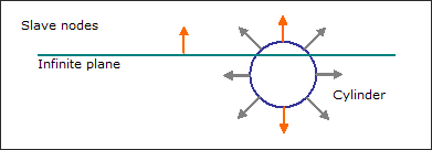
Fig 15: Incompatible kinematic conditions (no orthogonal directions of normals).
A 15600 mm.s-1 (56 km/h) initial velocity (/INIVEL) is applied to all nodes of the structure in the X direction at t = 0.3 s. This initial condition is defined in the D02 restart file (*_0002.rad, start time: 0.3 s), which is run after achieving the quasi-static equilibrium with gravity loading.
Option in restart file (*_0002.rad):
/INIV/TRA/X/1  initial translational velocities in the X direction
15600  of 15600 mm/s
1 265130 on node 1 to 265130 (/INIV/TRA/X/1)
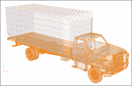
Fig 16: Selected nodes for the initial translational velocity of the truck (56 km/h) at t = 0.3 s.
Quasi-static Loading: Gravity Effect on Initial Static Equilibrium
The quasi-static solution of gravity loading on structure deformation is the steady state part of the dynamic response and describes the pre-loading case before the transient analysis. Thus, simulation is divided into two phases: quasi-static response (structure deformation under the gravity effect) and dynamic behavior (run and impact on the bump). he solution is obtained using the kinetic relaxation method.
Gravity is applied to all nodes of the model. A constant function defines the gravity acceleration in the Z direction versus time and is equal to -9810 mms-2. Gravity is activated with the /GRAV option.
The explicit time integration scheme assumes starting with nodal acceleration computation. It is very efficient for simulating dynamic loadings. Nevertheless, quasi-static simulations via a dynamic resolution method need to minimize the dynamic effects in order to converge towards static equilibrium. Among the usual methods employed, the kinetic relaxation method is quite effective and is activated in the Engine file (*_0001.rad) using /KEREL. All velocities are set to zero each time the kinetic energy reaches a maximum value.
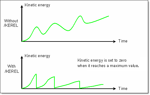
Fig 17: Kinetic relaxation method using the /KEREL option.
Simulation Results and Conclusions
Animation of the passing over the speed bump:
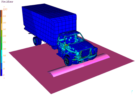
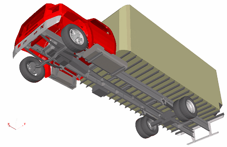
Fig 18: Distribution of von Mises stress on the model during bump passage.
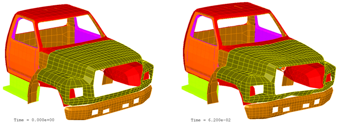
Fig 19: Cab deformation (initial state and after bump passage).