|
»Click here to display Table of Contents«
|

16.2 - IMPLICIT Solver |

|

|

|

|
|
16.2 - IMPLICIT Solver |
|
|
|

|
|
»Click here to display Table of Contents«
|
16.2 - IMPLICIT Solver |
|
|
|
|
|
16.2 - IMPLICIT Solver |
|
|
|
|
TitleIMPLICIT solver |
|
||||||||||||||||||
Number16.2 |
|||||||||||||||||||
Brief DescriptionA dummy is sat down via gravity using the implicit approach (static). |
|||||||||||||||||||
Keywords
|
|||||||||||||||||||
RADIOSS Options
|
|||||||||||||||||||
Input FileLinear_implicit_model: <install_directory>/demos/hwsolvers/radioss/16_Dummy_Positioning/IMPLICIT_solver/Linear/SEAT_IMPL_LIN* Nonlinear_implicit_model: <install_directory>/demos/hwsolvers/radioss/16_Dummy_Positioning/IMPLICIT_solver/Nonlinear/
|
|||||||||||||||||||
Technical / Theoretical LevelAdvanced |
|||||||||||||||||||
The main advantages of implicit resolution are:
| • | Unconditional stable scheme |
| • | Large time step |
| • | Treatment of the static problem |
However, the implicit algorithm uses a global resolution which requires convergence for each time step and has low robustness in comparison to the explicit (null pivots, divergence for high nonlinearities, etc.).
The implicit methods result in solving a linear system for each time step, which is relatively expensive but enables a large time step: few expensive calculations. The explicit method treats linear or nonlinear systems depending on the problem. It is less expensive and faster for each step, but requires short time steps to ensure stability of the scheme that has many inexpensive cycles.
| • | Implicit integration scheme: Newmark |
This scheme is unconditionally stable, the stability condition being independent of the time step choice. See the RADIOSS Theory Manual for further information about the Newmark scheme.
RADIOSS has a linear and a nonlinear solver. Only static computations are available and loading should be defined as a monotonous increasing time function for nonlinear analysis.
The main computational methods available in RADIOSS:
| • | Cholesky (direct method, linear solver) |
| • | Preconditioned Conjugate Gradient (linear solver) |
| • | Modified Newton-Raphson method (nonlinear solver) |
The precondition methods for linear solver available in RADIOSS:
| • | No preconditioned |
| • | Diagonal Jacobi |
| • | Incomplete Cholesky |
| • | Stabilized incomplete Cholesky |
| • | Factored Approximate Inverse (by default) |
You should define the tolerance and stop criterion for the linear and nonlinear solver (residual).
Strategies of resolution for nonlinear static computation/time step control:
| • | Iterations number limit for updating stiffness matrix |
| • | Convergence iterations number for increasing time step |
| • | Convergence iterations number for decreasing time step |
| • | Increase time step factor |
| • | Decrease time step factor |
| • | Minimum time step |
| • | Maximum time step |
| • | Initial time step |
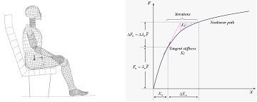
The nonlinear solver uses the modified Newton-Raphson method and the resolution is based on sparse iterative techniques.
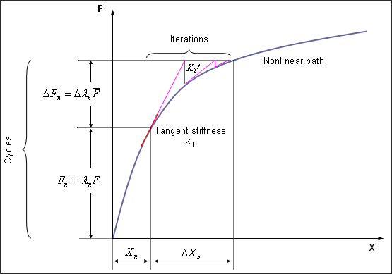
Fig 19: Newton-Raphson resolution in the case of load control technique.
The modified Newton-Raphson method is based on maintaining the tangent matrix for all iterations and can be combined with the line search acceleration technique for accelerating convergence.
Piloting techniques available in RADIOSS:
| • | Displacement norm control |
| • | Arc-length control |
An automatic time step control is used.
This example deals with two implicit analysis':
| • | A static linear computation (loading by gravity), |
| • | A static nonlinear computation (three computations are performed: dummy positioning using an imposed displacement, followed by a concentrated load and a gravity loading). |
An adapted modeling methodology is set up for each analysis. Contact with the different interfaces depends on the computations taken into account and then the material can be updated.
The goal for this analysis is to propose a modeling method for different loading cases, with specific input data used in the implicit strategies. The studies by linear implicit and nonlinear implicit using imposed displacement are no longer comparable with results obtained by explicit due to the different physical approaches. Comparisons are only valid for the positioning by gravity loading.
Type 7 interface uses nonlinear algorithms to check contact. Thus, in order to be used in a linear solver, it is replaced by a type 2 tied interface which creates kinematic conditions between slave nodes and master surfaces. Gravity loading is studied.
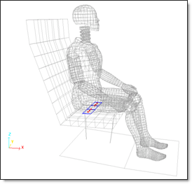
Fig 20: Type 2 tied interface linear contact for dummy / seat cushion modeling.
The visco-elastic law 35 (generalized Kelvin-Voigt model) describing the foam of a seat is converted into a linear plastic law 1 (properties are maintained):
| • | Young’s modulus: 0.2 MPa |
| • | Poisson’s ratio: 0 |
| • | Density: 4.3 x 10⁻¹¹ k g/l |
You can select BATOZ formulations for the shell elements and HA8 formulations using 2x2x2 integration points for the brick elements.
The linear implicit methods used are:
| Implicit type: | Static linear |
| Linear solver: | Direct Cholesky |
| Precondition method: | Factored Approximate Inverse |
| Stop criteria: | Relative residual of preconditioned matrix |
| Tolerance: | 10-6 |
The implicit options used in the Engine file are:
/IMPL/PRINT/LIN/-1 |
Printout frequency for linear iteration |
/IMPL/SOLVER/3 |
Solver method |
/IMPL/LINEAR |
Static linear computation |
Results
Only one animation corresponds to the static solution.
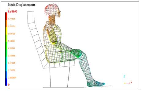
Fig 21: Linear static implicit solution of gravity loading (type 2 interface is used).
It should be noted that this modeling contact slightly modifies the problem which is no longer comparable with the previous explicit models.
Table 1: Indication of time computation.
|
Explicit Solver - |
Implicit Solver – |
|---|---|---|
Normalized CPU |
170 |
1 |
The modeling methodology defined in the explicit studies is maintained (visco-elastic material law, type 7 interface, etc.). Brick elements are modeled by default element formulation.
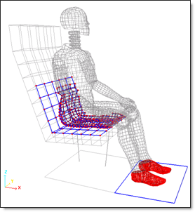
Fig 22: Nonlinear contact modeling with self-impacting type 7 interface.
In addition to the constant gravity load, an imposed displacement along the Z-axis is applied on the master node of the global rigid body covering the dummy. This approach allows computation to converge and the rigid body modes to be removed (no null pivot). An input curve for the imposed displacement is required. The boundary conditions on master node 14199 are: 110 111.
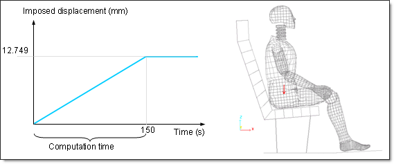
Fig 23: Imposed displacement along the Z-axis as a monotonous increasing time function.
The nonlinear implicit parameters used are:
| Implicit type: | Static nonlinear |
| Nonlinear solver: | Modified Newton |
| Stop criteria: | Relative residual in force |
| Tolerance: | 0.01 |
| Update of stiffness matrix: | 5 iterations maximum |
| Time step control method: | Arc-length method and "line-search" |
| Initial time step: | 5 s |
| Minimum time step: | 0.01 s |
| Maximum time step: | no |
| Desired convergence iteration number: | 6 |
| Maximum convergence iteration number: | 20 |
| Decreasing time step factor: | 0.8 |
| Maximum increasing time step scale factor: | 1.1 |
| Arc-length: | Automatic computation |
| Spring-back option: | no |
Implicit parameters are set in the Engine file with the options beginning with /IMPL/.
The implicit options used are:
/IMPL/PRINT/NONLIN/-1 |
Printout frequency for nonlinear iteration |
/IMPL/SOLVER/3 |
Solver method (solve Ax=b) |
/IMPL/NONLIN |
Static nonlinear computation |
/IMPL/DTINI |
Initial time step determines the initial loading increment |
/IMPL/DT/STOP |
Min-Max values for time step |
/IMPL/DT/2 |
Time step control metho 2 - Arc-length+Line-search will be used with this method to accelerate and control convergence |
Due to the contact problem, the tolerance value (Tol) is set to 10-2 (default = 10-3).
Some options are not compatible with the implicit solver. Refer to RADIOSS Starter Input for more details about implicit options.
The last animation corresponds to the static solution.
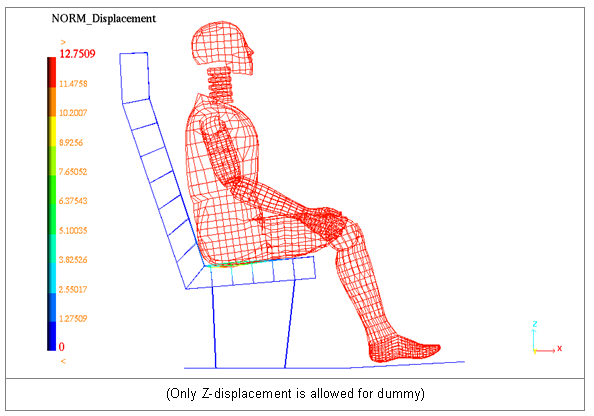
Fig 24: Nonlinear static implicit solution of the imposed displacement.
The Z-displacement of the dummy should not be considered as a result but as an input data (imposed displacement on the master node 14199).
Table 2: Time computation comparison between explicit and implicit computations:
|
Explicit Solver - |
Implicit Solver – |
|---|---|---|
Normalized CPU |
1.26 |
1 |
Number of cycles (normalized) |
56704 (1718) |
33 (1) |
The modeling methodology defined in the explicit studies is maintained. The gravity loading is taken into account by applying a constant concentrated load of 813.05N (dummy weight + added masses) on the master node of the rigid body, including the dummy. In order to remove the rigid body modes, the dummy is connected to fixed nodes via type 8 spring elements.
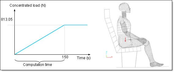
Fig 25: Concentrated load along the Z-axis as a monotonous increasing time function.
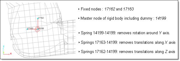
Fig 26: Springs type 8 defined for removing rigid body modes during implicit computation.
The properties of the general type 8 springs are:
| • | Linear elastic behavior |
| • | Mass = 1g |
| • | Inertia = 0.001 |
| • | Translational stiffness: TX = 1 N/mm |
TY = 1 N/mm
TZ = 1 N/mm
| • | Rotational stiffness: RX = 100 Mg.mm2/(s2.rad) |
RY = 100 Mg.mm2/(s2.rad)
RZ = 100 Mg.mm2/(s2.rad)
Implicit options are the same as the previous implicit problem; except for the initial time step is set to: 2s.
Table 3: Time computation comparison between explicit and implicit computations:
|
Explicit Solver - |
Implicit Solver – |
|---|---|---|
Normalized CPU |
3.07 |
1 |
Number of cycles (normalized) |
56704 (1090) |
52 (1) |
Z – displacement |
-12.75 mm |
-12.49 mm |
The modeling methodology defined in the implicit model is maintained using a concentrated load. Gravity loading is applied on the slave nodes and the master node of the rigid body, including the dummy. In order to remove the rigid body modes, the dummy is connected to fixed nodes via type 8 spring elements.
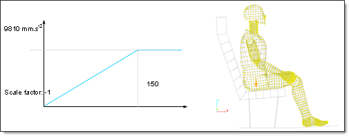
Fig 27: Gravity loading as a monotonous increasing time function.
Implicit options are the same as the previous implicit problem (initial time step is set to: 2s).
Table 4: Time computation comparison between explicit and implicit computations:
|
Explicit solver - |
Implicit solver – |
|---|---|---|
Normalized CPU |
2.53 |
1 |
Number of cycles (normalized) |
56704 (1090) |
52 (1) |
Z – displacement |
-12.75 mm |
-12.42 mm |
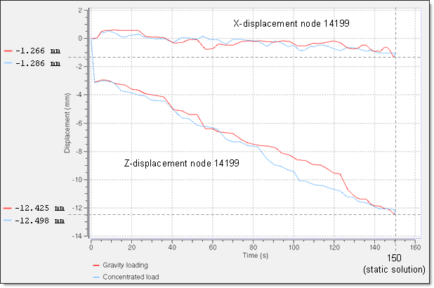
Fig 28: Convergence results of the X- and Z-displacement of master node 14199 (rigid body dummy) for the implicit models using gravity loading and concentrated load.
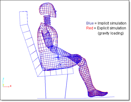
Fig 29: Final dummy position obtained using IMPLICIT (model using gravity loading) and EXPLICIT (model with gravity loading and kinetic relaxation).
This example brings awareness to the use of the RADIOSS implicit solver in resolving quasi-static problems. On the other hand, it illustrates different convergence acceleration techniques when an explicit solver is applied to the quasi-static problems. The advantages and drawbacks of the methods are compared.