|
»Click here to display Table of Contents«
|

6.2 - Fluid Flow |

|

|

|

|
|
6.2 - Fluid Flow |
|
|
|

|
|
»Click here to display Table of Contents«
|
6.2 - Fluid Flow |
|
|
|
|
|
6.2 - Fluid Flow |
|
|
|
|
TitleFuel tank - Fluid flow |
|
||||||||
Number6.2 |
|||||||||
Brief DescriptionFuel tank overturning with simulation of the fluid flow. The reversing tank is modeled using horizontally-applied gravity. The tank container is presumed without deformation and only the water and air inside the tank are taken into consideration using the ALE formulation. |
|||||||||
Keywords
|
|||||||||
RADIOSS Options
|
|||||||||
Input FileFluid_flow_gravity_1: <install_directory>/demos/hwsolvers/radioss/06_Fuel_tank/2-Tank_overturning/Fluid_flow_1/PFTANK* Fluid_flow_gravity_2: <install_directory>/demos/hwsolvers/radioss/06_Fuel_tank/2-Tank_overturning/Fluid_flow_2/PFTANK* |
|||||||||
Technical / Theoretical LevelAdvanced |
|||||||||
The fluid flow is studied during the fuel tank overturning. This example uses the ALE (Arbitrary Lagrangian Eulerian) formulation and the hydrodynamic bi-material law (/MAT/LAW37) to simulate interaction between water and air. The tank container is presumed without deformation and it will not be modeled.
A rectangular tank is partially filled with water, the remainder being supplemented by air. The tank turns once around itself on the Y-axis. The overturning is achieved by defining a gravity field in the X direction, which is parallel to the liquid gas interface. All gravity is applied in other directions. The initial distribution pressure is already known and supposed homogeneous. The tank dimensions are 460 mm x 300 mm x 10 mm.
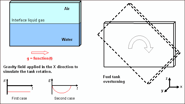
Fig 7: Problem description.
The example deals with two loading cases: an instantaneous rotation of the fuel tank by 90 degrees (gravity function 1) and a progressive rotation (gravity function 2).
The main material properties for the ALE bi-phase air-water are:
| • | Air density: 1.22x10⁻⁶ g/mm3 |
| • | Water density: 0.001 g/mm3 |
| • | Gas initial pressure: 0.1 MPa |
The bi-material air-water is described in the hydrodynamic material law (/MAT/LAW37). See previous section for information about this law, including full input data.
This loading case does not require a tank container mesh and the model, air and water are only comprised of the brick element using an ALE formulation.
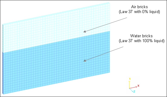
Fig 8: Air and water mesh (ALE bricks).
Using the ALE formulation, brick mesh is only deformed by the tank deformation, the water flowing through the mesh. The Lagrangian shell nodes still coincide with the material points, while the elements are deformed with the material: this is the Lagrangian mesh. For the ALE mesh, nodes on boundaries are fixed to remain on the border, while the interior nodes are moved.
Regarding the ALE boundary conditions (/ALE/BCS), constraints are applied on:
| • | Material velocity |
| • | Grid velocity |
All nodes inside the border have grid and material velocities fixed in the Z direction; the nodes on the left and right sides have a material velocity fixed in the X and Z directions, while the nodes on the high and low sides have a material velocity fixed in the Y and Z directions. The grid velocity is fully fixed on the border, just as the material velocity is fixed on the corners.
A function defines gravity acceleration in the X direction compared with time in order to simulate the rotation effect. Gravity is activated by /GRAV. Two cases are studied depending on the acceleration function selected:
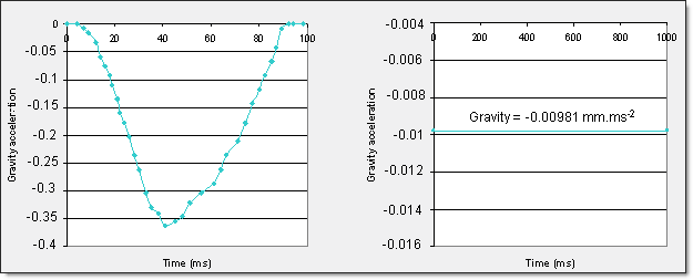
| Fig 9: Variable acceleration function 1 | Fig 10: Constant acceleration function 2 |
Gravity is considered for all nodes.
| • | Both ALE materials air and water must be declared as ALE using /ALE/MAT. Lagrangian material is automatically declared as Lagrangian. |
| • | The /ALE/GRID/DONEA option activates the J. Donea grid formulation in order to compute grid velocity. See the RADIOSS Theory Manual for further explanation about this option. |
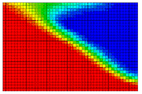
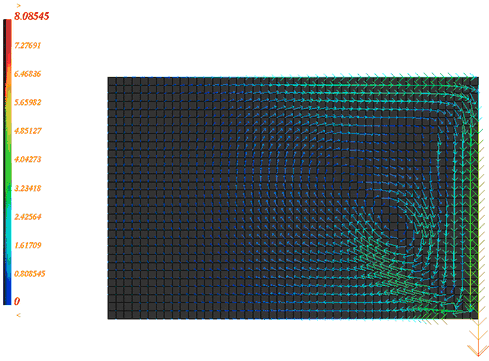
Model with Constant Acceleration |
Time = 170 ms |
Density
|
|
Velocity
|
|
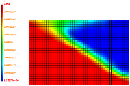
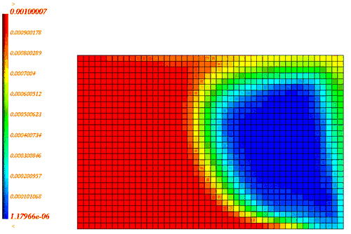
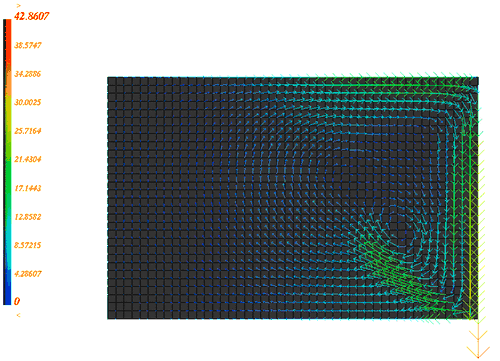
Model with Constant Acceleration |
Time = 280 ms |
Density
|
|
Velocity
|
|
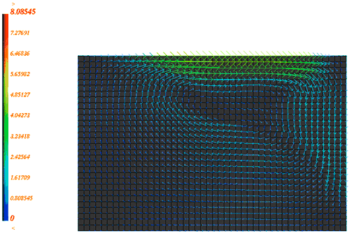
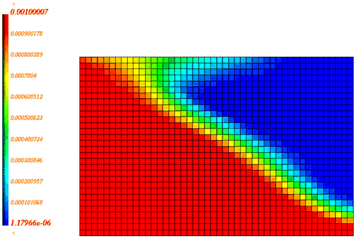
Model with Variable Acceleration |
Time = 50 ms |
Density
|
|
Velocity
|
|
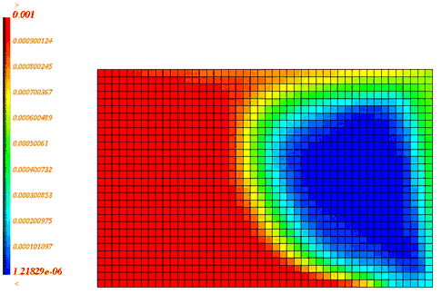
Model with Variable Acceleration |
Time = 70 ms |
Density
|
|
Velocity
|
|
This example studied hydrodynamic bi-material using Law 37 in RADIOSS, using ALE and Eulerian formulations. The application of boundary conditions in ALE formations and handling the fluid-structure interaction were discussed. Furthermore, the results obtained correctly represent the physical problem.