|
»Click here to display Table of Contents«
|

Example 7 - Pendulums |

|

|

|

|
|
Example 7 - Pendulums |
|
|
|

|
|
»Click here to display Table of Contents«
|
Example 7 - Pendulums |
|
|
|
|
|
Example 7 - Pendulums |
|
|
|
|
The purpose of this example is to simulate the oscillation and wave propagation of a group of pendulums, arranged in a line, when impacted at one end. The material is described as being elastic. Two models are used to simulate two different physical problems:
| • | The 2D model represents the infinite cylindrical mass for pendulums |
| • | The 3D model is necessary for determining the spherical mass |
The quality of the model first depends on how contact is managed. For the 2D model, a simple type 5 interface with a plane facet is used. For the 3D model, however, a type 16 interface using the Lagrange Multipliers method is used.
TitlePendulums |
|
||||||||
Number7.1 |
|||||||||
Brief DescriptionFive pendulums in line, initially in contact with each other, are struck by a sixth one. The shock wave and oscillating motion are observed. |
|||||||||
Keywords
|
|||||||||
RADIOSS Options
|
|||||||||
Compared to / Validation Method
|
|||||||||
Input FileTri-dimensional_analysis: <install_directory>/demos/hwsolvers/radioss/07_Pendulums/3D_model/PENDULUMS_3D* Bi-dimensional_analysis: <install_directory>/demos/hwsolvers/radioss/07_Pendulums/Plan_strain_model/PENDULUMS_2D* |
|||||||||
Technical / Theoretical LevelMedium |
|||||||||
The purpose of this example is to study the shock wave propagation and the momentum transfer through several bodies, initially in contact with each other, subjected to multiple-impact. The process of collision and the energetic behavior upon impact are delineated using a tri-dimensional model. A plane strain assumption can be used as a compliment to this study, whereby a bi-dimensional model using fine mesh enables shock wave propagation and the mechanics contact to be shown in a qualitative manner.
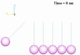
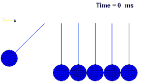
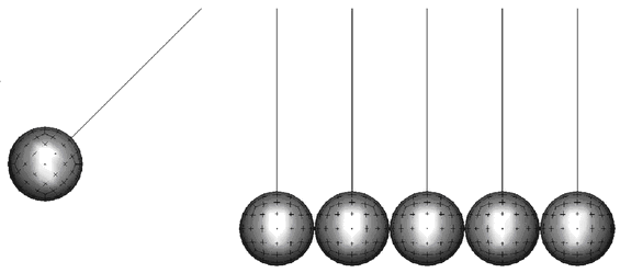
A metal ball strikes a line of five balls, initially in contact with each other. The momentum is transferred from pendulum to pendulum until reaching the last one at the opposite end. The system is subjected to gravity. This results in the end pendulums alternate oscillating for half the time period.
The following system is used: mm, ms, g, N, MPa.
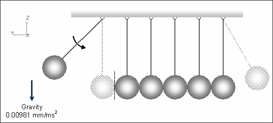
Fig 1: Description of the problem.
The left pendulum has an initial angle of 45 degrees in relation to the vertical. The material used is aluminum alloy which behaves like a linear elastic law (/MAT/LAW1) during impact.
The properties are defined as follows:
| • | Young’s modulus: 70000 MPa |
| • | Poisson’s ratio: 0.33 |
| • | Density: 0.0027 g.mm-3 |
The geometrical characteristics of the balls and trusses are:
| • | Truss: |
- Length: 124.6 mm
| • | Ball: |
- Radius: 25.4 mm (massball = 182.5g)
Two approaches 2D and 3D are used to provide complementary simulation results.
Brick and thick shell elements are used to create the 3D model for balls. The quadratic 16-node thick shell element is used to model the external surface of the balls. However, the core of each ball is modeled using 8-node solid elements.
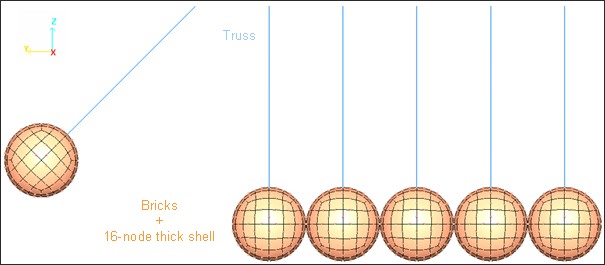
Fig 2: Tri-dimensional mesh in initial state.
The modeling technique used enables to ensure contact between the quadratic surfaces.
Figure 3 shows the mesh used for balls. The mesh uses a hypercube mesh topology combining brick and 16-node thick shell elements.
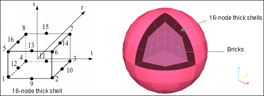
Fig 3: Mesh for balls (brick and 16-node thick shell).
The type 16 interface using the Lagrange Multipliers method is employed to model contacts between the nodes and the quadratic elements’ surface. An interface must be defined for each ball (five interfaces).
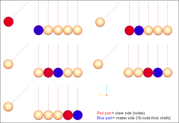
Fig 4: Slave nodes and master surfaces defined for the type 16 interface.
No gap is required for the type 16 interface, enabling the contact condition to be exactly satisfied.
Gravity is applied to all nodes. A function defines the gravity acceleration in the Z direction compared with time. Gravity is activated by the /GRAV option.
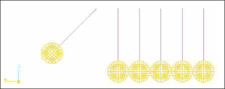
Fig 5: Gravity loading (-0.00981 mm.ms-2 ).
The upper extremities of the trusses are fixed in Y and Z translations and in Y and Z rotations.
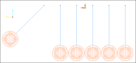
Fig 6: Boundary conditions on the upper extremities of trusses.
By adopting a plane strain approach, a 2D model is used (N2D3D = 2 in the /ANALY option set in the input file). The plane strain analysis defines the X-axis as the plane strain direction.
The mesh consists of 2D solid elements (quads). The dimension of the quad is about 0.5 mm for balls.
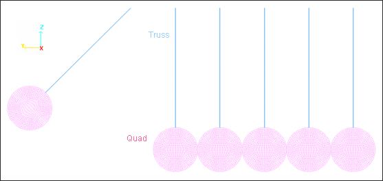
Fig 7: 2D mesh in the initial state.
Normal vectors of quad elements should have the same orientation to avoid negative volumes. Quad elements undergo a type 14 general solid property.
The contact between the external segments of the quads is modeled five times using a type 5 interface.
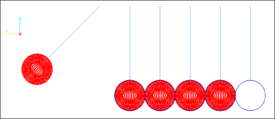
Fig 8: Master segments and slave nodes defined for type 5 interfaces.
Type 5 interface uses the Penalty method for a master segment contact (blue side) to the slave node (red side). The gap is set to 0.1 mm as the initial interval between the masses. The contact is sliding using a Coulomb friction coefficient that is equal to zero.
Type 7 general interface is not available in a 2D analysis.
The upper extremities of the trusses are fixed in Y and Z translations. The 2D conditions are automatically taken into account with N2D3D = 2 in /ANALY.
Gravity is applied to all nodes. A constant function (-0.00981 mm.ms-2) defines the gravity acceleration in the Z direction compared with time. Gravity is activated by /GRAV.
For the 2D analysis, the rigid body /RBODY option is not available.
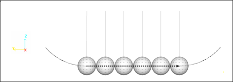
For the purpose of this example, the following numbers are assigned to the balls:
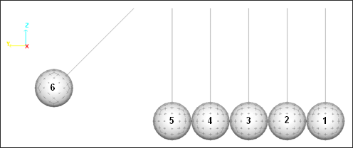
Fig 9: Ball numbers.
Figure 10 shows the kinetic energy variation of the model. When considering energy, the system behaves as a simple pendulum.
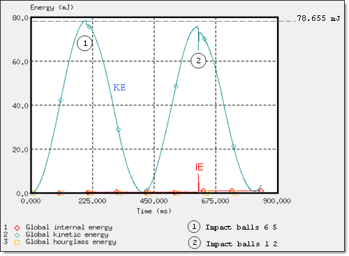
Fig 10: Global energy assessment.
When the pendulum mass is released at time t=0, the No. 6 end ball has maximum potential energy and null kinetic energy. Ball 6 achieves maximum velocity before striking the five other pendulums. For a moderate case that is without loss, you have:
![]()
Where, h is the vertical displacement of the ball’s center, V is the velocity and m is the mass.
The maximum kinetic energy is reached for: |
h = hmax = I(1 - cos(45)) = 43.934 mm |
Analytical solution: |
EKINETICmax = mghmax = 182.5 * 0.00981 * 43.934 = 78.656 mJ |
Simulation results: |
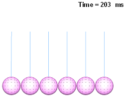
EKINETICmax = 78.655 mJ (time = 203.33 ms, impact balls 6 and 5) |
|
EKINETICmax = 72.478 mJ (time = 612.5 ms, impact balls 1 and 2) |
Maintaining the kinetic energy in the system is not entirely satisfactory, due to the energy contact being dissipated during impact.
The two extreme pendulums alternate, oscillating for half of the time period. The velocity of the middle balls in comparison to time is shown in Fig 11.
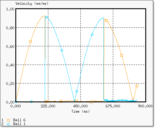
Fig 11: Velocity transmission between the end balls 1 and 6.
Velocity is transferred from pendulum to pendulum until reaching the end one.
The relative motion of a simple pendulum can be described using the equation:
![]()
where, ![]() is the system’s pulsation:
is the system’s pulsation:

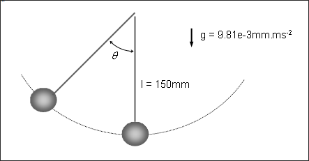
Fig 12: Pendulum motion.
Such analytical equation can be corroborated with regard to the end balls No. 1 and 6.
Rotations ![]() and rotational accelerations
and rotational accelerations ![]() are indicated from the nodes located at the upper end of the trusses.
are indicated from the nodes located at the upper end of the trusses.
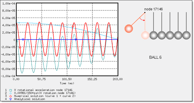
Fig 13: Verification of the equation ![]() for ball 6.
for ball 6.
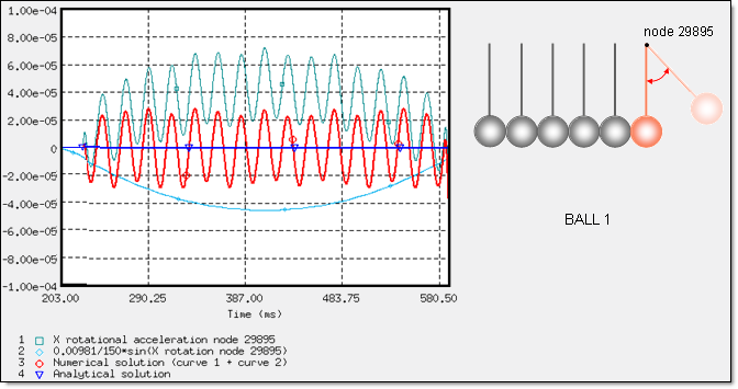
Fig 14: Verification of the equation ![]() for ball 1.
for ball 1.
The numerical results have an average correlation in relation to the analytical solution, due to the dynamic response of the nodal acceleration saved in the Time History.
Lets consider the interval [203,33 ms and 204,11 ms] where multiple impacts occur from balls No. 6 to 1.
As shown in Fig 15, the internal energy stored in the system is released after each impact, in line with the defining balls linear material law. The kinetic energy is transferred from pendulum to pendulum.
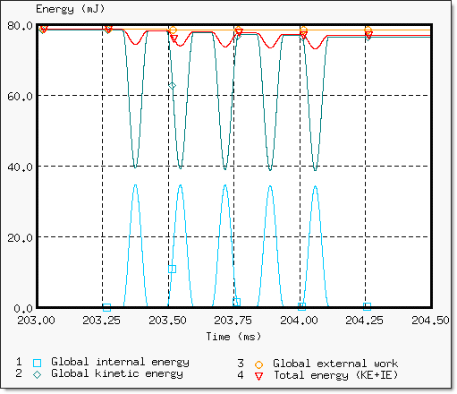
Fig 15: Global energy assessment during multiple impacts.
The 16-node thick shells are elements, which do not suffer hourglass deformation. Therefore, the low kinetic energy lost during multiple impact is due to the dissipated contact energy (-2.47mJ). The external work of the gravity remains constant (78.655mJ).
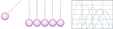
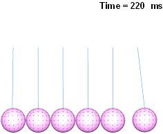
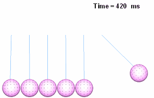
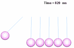
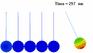
The following animations separately illustrate:
| • | the motion of the pendulums |
| • | the kinetic energy transmission |
| • | the stress wave propagation |
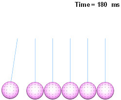
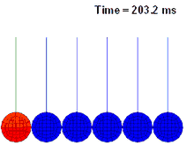
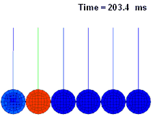
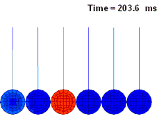
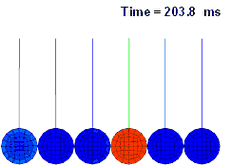
Balls Motion (Oscillations) |
|
|---|---|
|
|
|
|
|
|
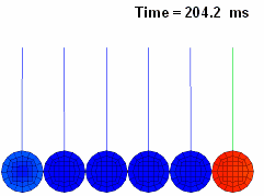
Momentum transmission from pendulum to pendulum (cutting plane X = 0):
Velocity Norm |
|
|---|---|
|
|
|
|
|
|
|
|
| Time for total transmission: 0.78 ms | Maximum = 1.08588 m.s-1. |
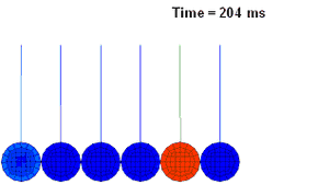
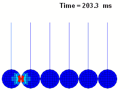
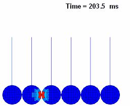
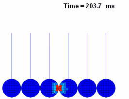
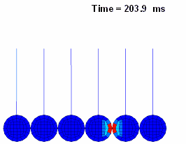
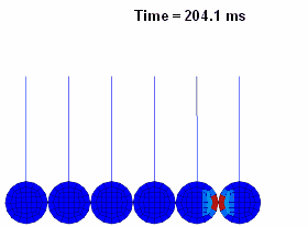
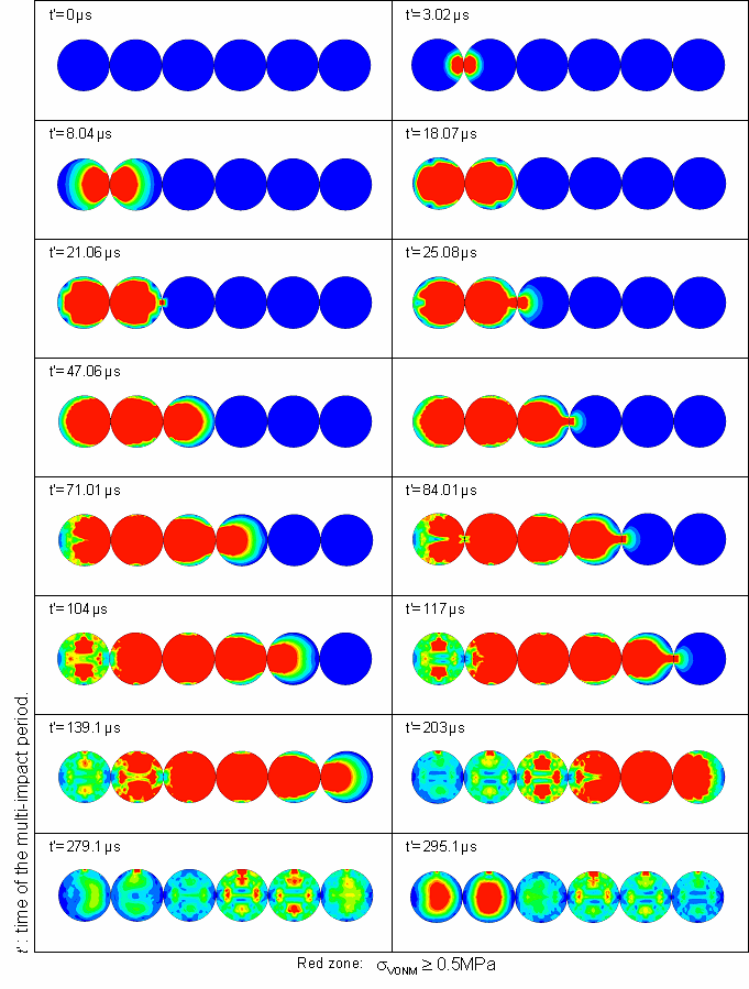
Shock wave propagation during multiple impact (cutting plane X=0):
von Mises Stress Wave |
|
|---|---|
|
|
|
|
|
|
| Time for transmission: 0.78 ms | Maximum = 17.7062 MPa. |
In this section covers the mechanics contact across a 6-ball chain.
The plane strain assumption changes the physical problem. Nevertheless, this case study is an interesting example of a system undergoing several shocks.
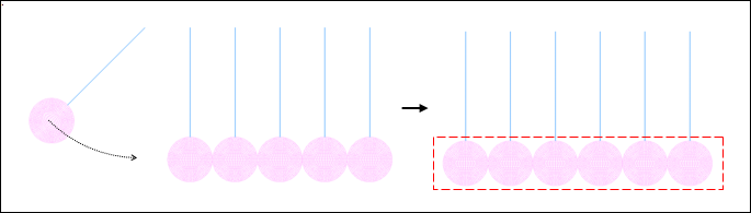
Fig 16: A 6-ball chain system.
The force between balls compared with time is shown in Fig 17. Existence of a time interval where forces’ contacts are not at zero.
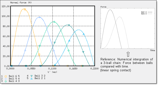
Fig 17: Forces’ contact between balls compared with time (contact starts at t’=0 ms).
This process leads to multiple impacts. It corroborates the experimental observations, where the theory was well estimated. Based on an Impulse Correlation Ratio (ICR), a regularized system of an N-ball chain using an elastic contact spring gives similar results.
| • | Reference results: [V. Acaray, B. Brogliato/Second MIT Conference on Computational Fluid and solid Mechanics] |
von Mises stress wave propagation from ball to ball during the multiple impact period (isostep values):
The impact between several pendulums in line was studied using RADIOSS. Two models representing physical problems were studied:
(i) a global analysis using a relatively coarse mesh with 3D elements
(ii) a 2D model using a fine mesh
In the first case, the energy assessment and the wave propagation are studied. The mesh used is not fine enough for studying the contact effects, due to the fact that 3D represents a high cost model and using a fine mesh dramatically increases the computation time. The results are compared to an analytical solution where the pendulum system is assimilated to a simple pendulum.
The 2D analysis concentrates on contact between the balls. There still exists an analytical solution though for a chain of three balls, but which can be generalized for the purpose of this example. The results obtained by simulation and theory demonstrate the validity of the numerical results obtained by RADIOSS.