Summary
Precise data for high strain rate materials is necessary to enable the accurate modeling of high-speed impacts. The high strain rate characterization of materials is usually performed using the split Hopkinson Pressure Bar within the strain rate range 100-10000 s-1. Using the one-dimensional analysis of the Hopkinson bar experiment, it is assumed that the object deforms under uni-axial stress, the bar object interfaces remain planar at all times, and the stress equilibrium in the object is achieved using travel times. The RADIOSS explicit finite element code is used to investigate these assumptions.
Title
Split Hopkinson pressure bar testing
|
|
Number
8.1
|
Brief Description
The high strain rate tensile behavior of the 7010 aluminum alloy is studied using the Hopkinson pressure bar technique (stress wave).
|
Keywords
| • | Axisymmetrical analysis and quad elements |
| • | High strain rate and Split Hopkinson Pressure Bar (SHPB) |
| • | Wave propagation and stress pulse |
|
RADIOSS Options
| • | Axisymmetrical analysis (/ANALY) |
| • | Boundary conditions (/BCS) |
|
Compared to / Validation Method
|
Input File
High_strain_rate: <install_directory>/demos/hwsolvers/radioss/08_Hopkinson_Bar/High_strain_rate/SHPB_H*
Low_strain_rate: <install_directory>/demos/hwsolvers/radioss/08_Hopkinson_Bar/Low_strain_rate/SHPB_L*
|
Technical / Theoretical Level
Advanced
|
Overview
Aim of the Problem
In order to model and predict the behavior of material during impact, the responses at very high strain rates should be studied. The Split Hopkinson Bar is an inexpensive device for performing high strain-rate experiments [1]. This equipment consists of four long pressure bars:
The object is sandwiched between the transmission and the incident bar. Assuming that the wave propagation in the bar is non-dispersive, the force and displacement upon contact between the bar and the object can be obtained from the strains measured through experience. In this example, the dynamic tensile behavior, achieved through experience of the 7010 aluminum alloy with a Split Hopkinson Pressure Bar (SHPB) is compared to numerical simulations. Two cases are studied at the strain rates of 80 s-1 (low rate) and 900 s-1 (high rate) respectively. At high strain rates, experience shows that the stress flow significantly increases by more than 30% with the strain rate increasing; thus demonstrating strain rate dependence in aluminum alloys in general. For the strain rates’ range applied here, an existing Johnson-Cook model is used to describe the stress flow as a strain and strain rate function. Failure is not taken into account.
Physical Problem Description
The Split Hopkinson Pressure Bar technique corresponds to a high strain rate deformation of the aluminum alloy at high stress. Figure 1 shows a diagram of the basic Hopkinson bar setup. It consists of two cylindrical bars of the same diameter, respectively called Input and Output bars.
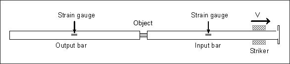
Fig 1: Hopkinson bar device.
The objects material undergoes an isotropic elasto-plastic behavior which can be reproduced using a Johnson-Cook model (/MAT/LAW2). The steel bars and the striker follow a linear elastic law (/MAT/LAW1).
The following system is used: mm, ms, g, N, MPa.
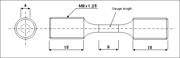
Fig 2: Object geometry and cross-section (dimensions in mm).
Johnson-Cook Model
The Johnson-Cook model describes the stress in relation to the plastic strain and the strain rate using the following equation:
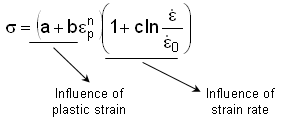
where:
 is the strain rate
0 is the reference strain rate
 p is the plastic strain (true strain)
a is the yield stress
b is the hardening parameter
n is the hardening exponent
c is the strain rate coefficient
The two optional inputs, strain rate coefficient and reference strain rate, must be defined for each material in /MAT/LAW2 in order to take account of the strain rate effect on stress, that is the increase in stress when increasing the strain rate. The constants a, b and n define the shape of the strain-stress curve.
In the documents entitled CRAHVI, G4RD-CT-2000-00395, D.1.1.1, Material Tests – Tensile properties of Aluminum Alloys 7010T7651 and AU4G Over a Range of Strain Rates, the behavior of the 7010 aluminum alloy can be described according to the relations:
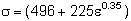 for strain rates below 80 s-1
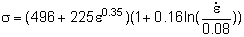 for strain rates exceeding 80 s-1 up to 3000 s-1
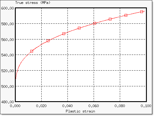
Fig 3: Yield curve of the Johnson-Cook model: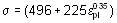
The material properties of the object are:
| • | Young’s modulus: 73000 MPa |
The material used for the bars and projectile is type 1 (linear elastic) with the following properties:
| • | Young’s modulus: 210000 MPa |
The geometrical characteristics of the bars and projectile are:
Bars:
Projectile:
High Strain Rate Test Method
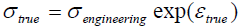
The object is screwed in between the incident and transmission bars. A stress pulse is introduced into the input bar through impact from a steel projectile on the steel disc attached to one end of the input bar. The impact generates a tensile wave which propagates along the input bar. Part of the wave is reflected and a part is transmitted via the object’s interface. The stress pulse continues through the object and into the transmitted bar. The wave reflections inside the sample enable the stress to be homogenized during the test. The strain associated with the output or transmitted stress wave is measured by the strain gauges on the output or transmitted bar. The strain gauges attached to the object gauge length, provide direct measuring of the true strain, and the true plastic strain in the object during the experiment. The transmitted elastic wave provides a direct force measurement to the bar object interfaces by way of the following relation:
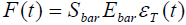
Where, Ebar is the modulus of the output bar, T is the strain associated with the output stress wave and the Sbar is the cross-section of the output bar.
If the two bars remain elastic and wave dispersion is ignored, then the measured stress pulses can be assumed to be the same as those acting on the object.
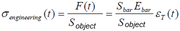
The engineering stress value in the object can be determined by the wave analysis, using the transmitted wave:
Engineering stress can also be found by averaging out the force applied by the incident that is the reflected and transmitted wave, as shown in the equation:
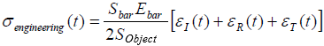
Where, I and R are the strains associated with input stress wave and T is the strain associated with output stress wave.
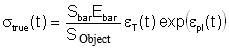
True stress in the object is computed using the following relation (refer to Example 11 - Tensile Test for further details):
The true strain rate is given by:

True stress and true strain are evaluated up to the failure point.
Interface 1: F1 = Sbar ( I(t) + R(t)) = SbarEbar(I(t) + R(t))
Interface 2: F2 = Sbar T(t) = SbarEbarT(t)
Balance in object: F1 = F2 ; 1(t) + R(t) = T(t)
Engineering stress in object: object (t) = F1 / Sobject = F2 / Sobject
Fig 4: 1D analysis.
Strain Rate Filtering
Because of the dynamic load, strain rates cause high frequency vibrations which are not physical. Thus, the stress-strain curve may appear noisy. The strain rate filtering option enables to dampen such oscillations by removing the high frequency vibrations in order to obtain smooth results. A cut-off frequency for strain rate filtering (Fcut) is used with a value less than half of the sampling frequency (1/ This or 1/Tsampling) defined in the Engine file (*_0001.rad) using the /TFILE option. Refer to Example 11 - Tensile Test for further details.
The cut-off frequency is set at 100 kHz in this example.
Analysis, Assumptions and Modeling Description
Modeling Methodology
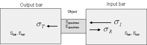
Taking into account the geometry’s revolution symmetry the material and the kinematic conditions, an axisymmetrical model is used (N2D3D = 1 in /ANALY set up in the Starter file). Y is the radial direction and Z is the axis of revolution.
The mesh is made of 12054 2D solid elements (quads). The quad dimension is about 2 mm.
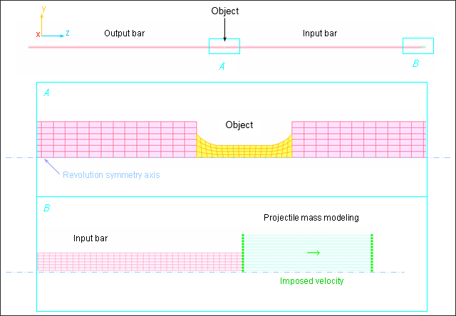
Fig 5: Mesh of the axisymmetrical model with imposed velocities on the top of the input bar.
RADIOSS Options Used
Low extremity nodes of the output bar are fixed in the Z direction. The axisymmetrical condition on the revolutionary symmetry axis requires the blocking of the Y translation and X rotation.
The projectile is modeled using a steel cylinder with a fixed velocity in the direction Z. The required strain rate is taken into account by applying two imposed velocities, 1.7 ms-1 and 5.8 ms-1 in order to produce strain rate ranges in the of 80 s-1 and 900 s-1 (low and high rates) object.
True Stress, True Strain and True Strain Rate Measurement from Time History
Fig 6: Nodes and quads saved for Time History.
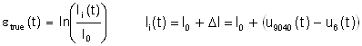
In the experiment, the strain gauge is attached to the object. In simulation, the true strain will be determined from 9040 and 6 nodes’ relative Z displacements (l0 = 3.83638 mm).
The true stress can be given using two data sources. The first methodology consists of using the equation previously presented, based on the assumption of the one-dimensional propagation of bar-object forces. The engineering strain t associated with the output stress wave is obtained from the Z displacement of nodes located on the output bar. The true plastic strain is extracted from the quads on the object, saved in the Time History file. True stress can also be measured directly from the Time History using the average of the Z stress quads 6243, 6244, 6224 and 6235. It should be noted that the section option is not an available option with the quad elements.
The strain rate can be calculated from either the true plastic strain of quads saved in /TH/QUAD or from the true strain true.
Table 1: Relations used in the analysis
|
High Rate Testing
|
True stress
|
|
Z stress average from quads saved in /TH
|
True strain
|
|
True strain rate
|

|

|
Simulation Results and Conclusions
The purpose of this test is to obtain the results observed in experiments with a Johnson-Cook model. The increase of stress is expected to equal approximately 30% compared to the low strain rate test.
Experimental Data
Experimental results show that the variation of the true tensile flow stress compared with the true strain is approximately equivalent to a strain rate between 80 s-1 and 100 s-1. The reference strain, in the Johnson-Cook model is set to 0.08 ms-1. At higher rates, the true flow stress increases significantly compared with the strain rate. The 7010 aluminum alloy exhibits an increase in the flow stress by a typical 30% at high strain rates (900 s-1 to 3000 s-1) compared to static values.
Results are given at the specific true strains of 0.02, 0.05 and 0.10. The influence of the strain rate on stress can be seen in Fig 7 [1].
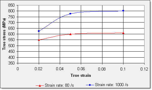
Fig 7: Variation of true stress compared with true strain for 7010 alloy using two different rates (experimental data).
For the test performed with a strain rate of 900 s-1, the flow stress reaches 850 MPa at a 0.25 strain.
Table 2: True stress at specific strains using both strain rates (experimental data).
|
Strain rate: 80 s-1
|
Strain rate: 900 s-1
|
True strain
|
0.02
|
0.05
|
0.1
|
0.02
|
0.05
|
0.1
|
0.25
|
True stress (MPa)
|
550
|
600
|
610
|
625
|
775
|
800
|
850
|
Johnson-Cook Model
Figure 8 shows the variation of true stress in time in relation to the wave propagation along the bars. Stresses are evaluated on the input bar, the object and the output bar.
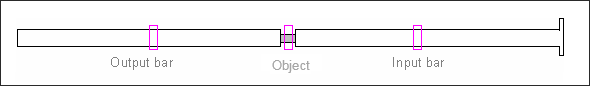
Fig 8: Stress measurement localizations.
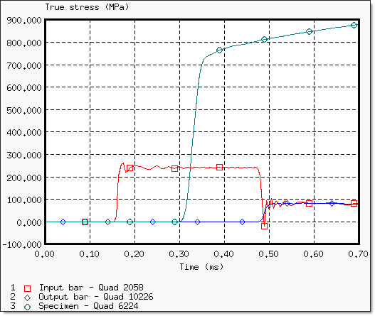
Fig 9: Stress waves in the input bar, the output bar and the object (imposed velocities = 5.8 ms-1 ).
The stress-time curve shows the incident, reflected and transmitted signals.
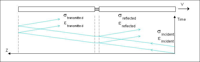
Fig 10: Diagram of SHPB showing the motion in time of the tensile pulse.
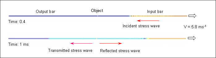
Fig 11: von Mises stress wave propagation along bars (imposed velocities = 5.8 ms-1 ).
The speed of wave, C along the bars is calculated using the relation:

C = 5189 ms-1
Where, E is the Young’s modulus and  is the density of the bars.
The time step element is controlled by the smallest element located in the object. It is set at 5x10⁻⁵ ms. The stress wave thus reaches the object in 0.77 ms and travels 0.26 mm along the bar for each time step. Obviously, it remains lower than the element length of the smallest dimension (0.88 mm).
An imposed velocity of 5.8 ms-1 produces a strain rate in the object of approximately 900 s-1, while a strain rate of approximately 80 s-1 is achieved using an imposed velocity of 1.7 ms-1. A simulation is performed for each velocity value. It should be noted that the study on low rates is more limited in time than on high rates due to the reflected wave generated on top of the output bar.
Figure 12 shows the true stress and true strain as a function of the strain rate.
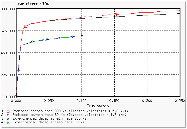
Fig 12: Variation of true stress with true strain for high and medium strain rates.
At a high strain rate (900/s), an increase in the flow stress is observed, being approximately 30% higher than the stress obtained for a low strain rate (80/s). The Johnson-Cook model used provides precise results compared with the experimental data.
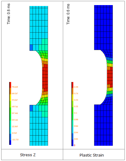
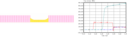
Fig 13: Stress Z and plastic strain on object at 0.6 ms.
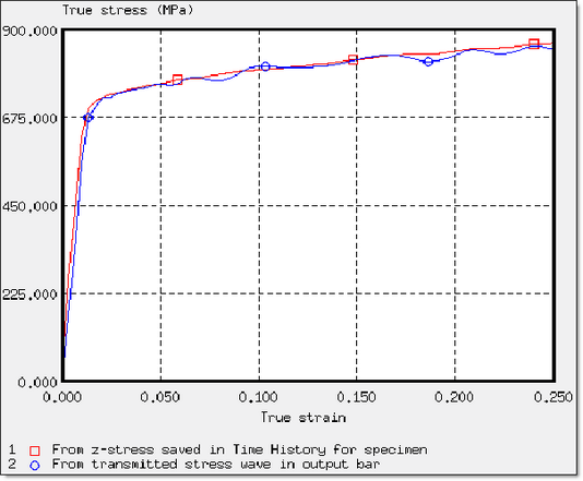
The true stresses determined from both methodologies are shown side-by-side. This validates the analysis based on a transmitted wave. Typical curves for a model having imposed velocities equal to 5.8 ms-1 are shown below:
True stress comparison in the object
|
|
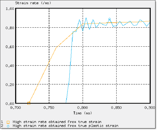
True strain rate in the object
(using both computations)
|
|
Either data sources used to evaluate the strain rate give similar results.
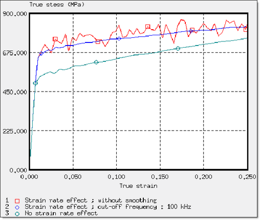
The following results show:
| • | the strain rate effect on stress, with or without the cut-off frequency for smoothing (100 kHz); |
| • | the influence of the strain rate coefficient (comparison with experimental data). |
Strain rate effect
|
|
Influence of the strain rate coefficient c
|
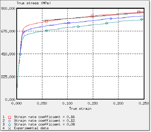
|
These studies are performed for the high strain rate model ( = 900 s-1).
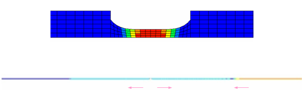
Figure 14 compares the distribution of the von Mises stress on the object, with and without the strain rate filtering at time t=0.6 ms.
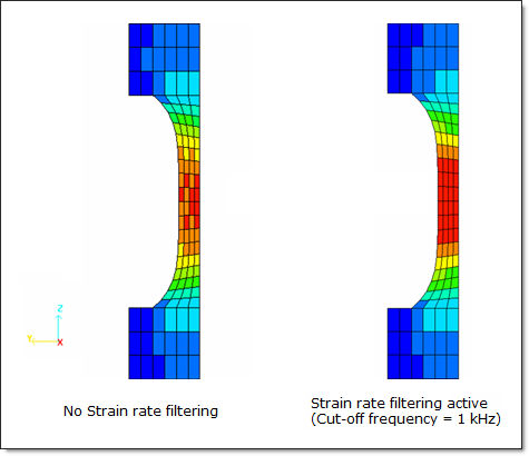
Fig 14: Comparison of the distribution of the von Mises stress at time t=0.6 ms.
More physical flow stress distribution is obtained using filtering. Explicit is an element-by-element method, while the local treatment of temporal oscillations puts spatial oscillations into the mesh.
Reference
[1] CRAHVI, G4RD-CT-2000-00395, D.1.1.1, Material Tests – Tensile properties of Aluminum Alloys 7010T7651 and AU4G Over a Range of Strain Rates.


