Title
Fuel tank - Fluid Structure Coupling
|
|
Number
6.1
|
Brief Description
Sloshing inside a fuel tank by simulating the fluid structure coupling. The tank deformation is achieved by applying an imposed velocity on the left corners. Water and air inside the tank are modeled with the ALE formulation. The tank container is described using a Lagrangian formulation.
|
Keywords
| • | Fluid structure coupling simulation, and ALE formulation |
| • | Shell and brick elements |
| • | Hydrodynamic and bi-phase liquid gas material (/MAT/LAW37) |
|
RADIOSS Options
| • | Boundary conditions (/BCS) |
|
Input File
Fluid_structure_coupling: <install_directory>/demos/hwsolvers/radioss/06_Fuel_tank/1-Tank_sloshing/Fluid_structure_coupling/TANK*
|
Technical / Theoretical Level
Advanced
|
Overview
Aim of the Problem
A numerical simulation of fluid-structure coupling is performed on sloshing inside a deformable fuel tank. This example uses the ALE (Arbitrary Lagrangian Eulerian) formulation and the hydrodynamic bi-material law (/MAT/LAW37) to model interaction between water, air and the tank container.
Physical Problem Description
A rectangular tank made of steel is partially filled with water, the remainder being supplemented by air. The initial distribution pressure is known and supposed homogeneous. The tank container dimensions are 460 mm x 300 mm x 10 mm, with thickness being at 2 mm.
Deformation of the tank container is generated by an impulse made on the left corners of the tank for analyzing the fluid-structure coupling.
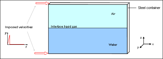
Fig 1: Problem description.
The steel container is modeled using the elasto-plastic model of Johnson-Cook law (/MAT/LAW2) with the following parameters:
| • | Young’s modulus: 210000 MPa |
| • | Hardening parameter: 450 MPa |
The material air-water bi-phase is described in the hydrodynamic bi-material liquid-gas law (/MAT/LAW37). Material law 37 is specifically designed to model bi-material liquid gas.
The equations used to describe the state of viscosity and pressure are:
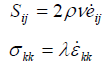

where, 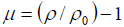
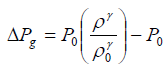
The equilibrium is defined by: Pl = Pg
Where, Sij is the deviatoric stress tensor and eij is the deviatoric strain tensor.
Material parameters are:
 | Liquid reference density: 0.001 g/mm3 |
| Cl | Liquid bulk modulus: 2089 N/mm2 |
| al | Initial mass fraction liquid proportion: 100% |
 | Shear kinematic viscosity (=  / /  ): 0.001 mm2/ms ): 0.001 mm2/ms |
 | Gas reference density: 1.22x10⁻⁶ g/mm3 |
| g | Shear kinematic viscosity (= /  ): 0.00143 mm2/ms ): 0.00143 mm2/ms |
 | Constant perfect gas: 1.4 |
| P0 | Initial pressure reference gas: 0.1 N/mm2 |
The main solid type 14 properties for air/water parts are:
| • | Quadratic bulk viscosity/linear bulk viscosity: 10-20 |
| • | Hourglass bulk coefficient: 10-5 |
Analysis, Assumptions and Modeling Description
Modeling Methodology
Air and water are modeled using the ALE formulation and the bi-material law (/MAT/LAW37). The tank container uses a Lagrangian formulation and an elasto-plastic material law (/MAT/LAW2).
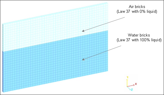
Fig 2: Air and water mesh (ALE brick elements).
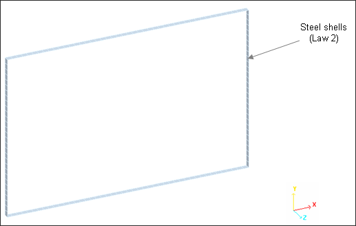
Fig 3: Tank container mesh (shell elements).
Using the ALE formulation, the brick mesh is only deformed by tank deformation the water flowing through the mesh. The Lagrangian shell nodes still coincide with the material points and the elements deform with the material: this is known as a Lagrangian mesh. For the ALE mesh, nodes on the boundaries are fixed in order to remain on the border, while the interior nodes are moved.
RADIOSS Options Used
Velocities (/IMPVEL) are imposed on the left corners in the X direction.
Table 1: Imposed velocity versus time curve
Velocity (ms-1)
|
0
|
5
|
0
|
0
|
Time (ms)
|
0
|
12
|
12.01
|
50
|
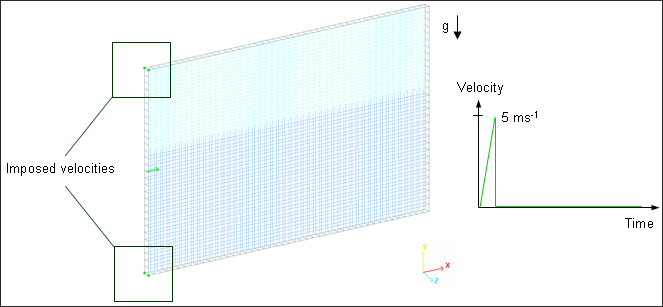
Fig 4: Kinematic condition: imposed velocities.
Regarding the ALE boundary conditions, constraints are applied on:
All nodes, except those on the border have grid (/ALE/BCS) and material (/BCS) velocities fixed in the Z-direction. The nodes on the border only have a material velocity (/BCS) fixed in the Z-direction.
Both the ALE materials air and water must be declared ALE using /ALE/MAT. Lagrangian material is automatically declared Lagrangian.
The /ALE/GRID/DONEA option activates the J. Donea grid formulation to compute the grid velocity. See the RADIOSS Theory Manual for further explanations about this option.
Simulation Results and Conclusions
Curves and Animations
Fluid – Structure Coupling
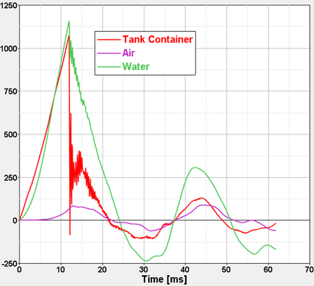
Fig 5: X – momentum variation for each part.
Kinematic conditions generate oscillations of the structure.
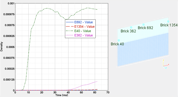
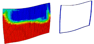
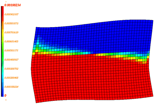
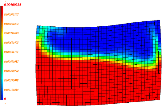
Fig 6: Density attached to the various brick elements.
Fluid Structure Coupling
|
Time = 0 ms
|
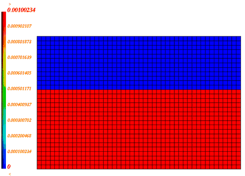
Density
|
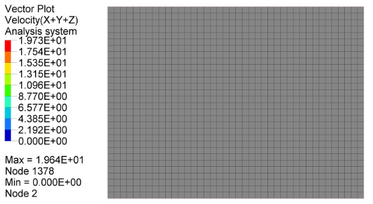
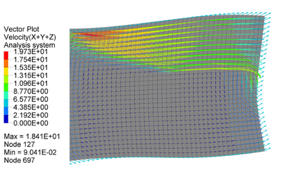
Velocity
|
Fluid Structure Coupling
|
Time = 12 ms
|
Density
|
Velocity
|
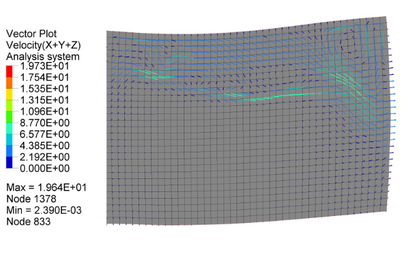
Fluid Structure Coupling
|
Time = 42 ms
|
Density
|
Velocity
|


