Model Element

Description

Constraint_Joint is used to specify an idealized connector between two bodies.

Constraint_Joint defines a set of lower pair constraints.  Physically, the joint consists of two mating surfaces that allow relative translational and/or rotational movement in certain specific directions only.  The surfaces are abstracted away, and the relationships are always expressed as a set of equations between points and directions on two bodies.

Format

<Constraint_Joint

    id             =     "integer"

    label          =     "Name of Joint"

    type           =     "CONSTANT_VELOCITY"

                         "CYLINDRICAL"

                         "FIXED"

                         "FREE"

                         "HOOKE"

                         "INLINE"

                         "INPLANE"

                         "ORIENTATION"

                         "PARALLEL_AXES"

                         "PERPENDICULAR"

                         "PLANAR"

                         "RACK_PINION"

                         "REVOLUTE"

                         "SCREW"

                         "SPHERICAL"

                         "TRANSLATIONAL"

                         "UNIVERSAL"

    i_marker_id     =    "integer"

    j_marker_id     =    "integer"

  [ pitch           =    "real" ]

  [ pitch_diameter  =    "real" ] >

/>

Attributes

id

The element identification number, (integer>0).  This is a number that is unique among all Constraint_Joint elements.

label

The name of the Constraint_Joint element.

i_marker_id

Specifies a Reference_Marker that defines the connection on the first body.  The body may be a rigid body, a flexible body, or a point body.  The parameter is required.

j_marker_id

Specifies a Reference_Marker that defines the connection on the first body.  The body may be a rigid body, a flexible body, or a point body.

type

Specifies the type of constraint connection between the i_marker and j_marker_id.

type may be one of the following:

"CONSTANT_VELOCITY"

"CYLINDRICAL"

"FIXED"

"FREE"

"HOOKE"

"INLINE"

"INPLANE"

"ORIENTATION"

"PARALLEL_AXES"

"PERPENDICULAR"

"PLANAR"

"RACK_PINION"

"REVOLUTE"

"SCREW"

"SPHERICAL"

"TRANSLATIONAL"

"UNIVERSAL"

The parameter is required.  See Comments 5-20 for more information about these joint types.

pitch

Defines the pitch of a screw joint.  The pitch defines the ratio between the translational and rotational motion in the screw joint.

The parameter is required only when TYPE = "SCREW_JOINT".

pitch_diameter

Defines the pitch diameter of the pinion gear a rack and pinion gear constraint.

The parameter is mandatory when TYPE = "RACK_PINION".

Comments

The internal reaction forces and moments at each Reference_Marker of the joint obey Newton’s third law of motion. Their magnitude and direction is such that they cancel each other out.

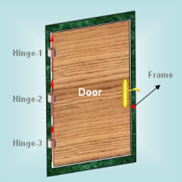
Consider a door connected to a frame as shown in Figure 1 below.

Figure 1: A simple system with redundant constraints

Both the door as well as the frame are assumed to be rigid.  Three hinges connect the door to the frame, allowing the door to open and close.  The hinges are modeled as revolute joints.  In this idealization, the hinges are assumed to be massless and rigid.  Each hinge allows rotation between the door and the frame about an axis, shown as a red arrow in Figure 1.

In this idealization, a few points should be noted:

If such a system is provided to MotionSolve, it will detect a redundancy in the constraints and remove the equivalent of two hinges from the model.  It will solve the system so that the correct motion is predicted.

The effect of removing two hinges from the solution process is to set their reaction forces to zero. Clearly, this is unexpected behavior.  In reality, all three hinges have reaction forces and torques. This is an issue with the idealization of the system.  If at least one of two bodies, the door or the frame, were made flexible, then more realistic reactions would be observed at each hinge.

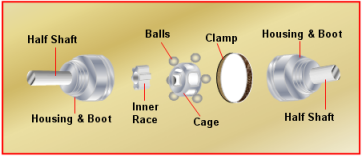
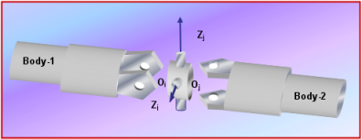
The constant velocity joint is a fairly complex subsystem.  It ensures that the angular speed of the output shaft is the same as the angular speed of the input shaft, regardless of their relative orientation.  The construction of a constant velocity joint is shown below in Figure 2.

Figure 2: A CONSTANT_VELOCITY joint

The detail in the constant velocity joint is abstracted away; all intermediate parts are ignored and the input-output relationship between the shafts is captured via a simple set of algebraic constraints.  Energy loss is not modeled.

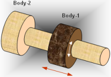
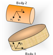
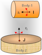
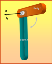
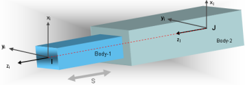
The cylindrical joint allows two degrees of freedom between the bodies it constraints.  Figure 4 shows a schematic of a cylindrical joint.  It allows a body (Body-1 in the Figure 3) to translate and rotate along a fixed axis defined on another body (Body-2 in Figure 3).

Figure 3: A CYLINDRICAL joint

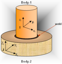
The fixed joint forces two bodies to move together as if they were welded together. No relative motion between the two bodies is allowed.  Figure 4 shows a schematic of a fixed joint.

Figure 4: A schematic of a FIXED joint

The location and orientation of any coordinate system "etched" on Body-2 is fixed with respect to any coordinate "etched" on Body-1.

The free joint is the exact opposite of the fixed joint. It does not restrict any motion between the two bodies it connects.  The free joint is typically used to define topology hierarchy, when joint (also known as relative) coordinates are used to internally represent the system.

Figure 5: A FREE joint

In a free joint, any coordinate system fixed on Body-2 can move in all possible ways with respect to a coordinate system fixed on Body-1.

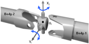
The image below shows a schematic of a HOOKE joint.  This joint constrains two Reference_Markers, I on Body-1 and J on Body-2 such that (a) their origins Oi and Oj remain superposed, and (b) the I marker x-axis is always perpendicular to the J marker y-axis.

A HOOKE joint

The HOOKE joint removes four degrees of freedom from a system.  Body-1 can rotate about the Xi axis and Body-2 can rotate about the Yi axis.  Relative translations are not allowed.  Physically, the HOOKE joint is identical to the UNIVERSAL joint.

This is a constraint primitive that requires that the origin of a Reference_Marker on Body-1 translate along the z-axis of a Reference_Marker placed on Body-2.  All rotations are allowed.  Figure 6 shows a schematic of an INLINE primitive.

Figure 6: A schematic of an INLINE joint

The inline primitive constrains two translational degrees of freedom.  It prohibits translation along the x- and y-axes of the Reference_Marker on Body-2.

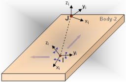
This is a constraint primitive that requires that the origin of a Reference_Marker on Body-1 (I in the figure below) to stay in the XY plane defined by the origin of the J Reference_Marker and its z-axis. Figure 7 shows a schematic of an INPLANE primitive.

Figure 7: A schematic of an INPLANE joint

The INPLANE primitive constrains one translational degree of freedom. It prohibits translation along the z-axis of the Reference_Marker J on Body-2.  All rotations are allowed.

Figure 8 shows a schematic of an ORIENTATION joint.  It requires that the orientation of a Reference_Marker on Body-1 (I in the figure below) always be the same as the orientation of a Reference_Marker on Body-2 (J in the figure below).

Figure 8: An ORIENTATION joint

The ORIENTATION joint removes three degrees of freedom; all of these are rotational.  All three translations of Body-1 with respect to Body-2 are allowed.

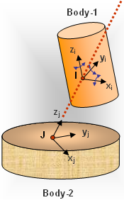
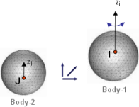
Figure 9 shows a schematic of a PARALLEL_AXES joint.  This joint constrains Body-1 such that the z-axis of a Reference_Marker (I in Figure 9) is always parallel to the z-axis of a Reference_Marker on Body-2 (J in the Figure 9).

Figure 9: A PARALLEL_AXES joint

The PARALLEL_AXIS joint removes two rotational degrees of freedom. Rotation of Body-1 is only allowed about the z-axis of the I Reference_Marker. All three translations are allowed.

Figure 10 shows a schematic of a PERPENDICULAR_AXES joint. This joint constrains Body-1 such that the z-axis of a Reference_Marker (I in Figure 10) is always PERPENDICULAR to the z-axis of a Reference_Marker on Body-2 (J in the Figure 10).

Figure 10: A PERPENDICULAR_AXES joint

The PERPENDICULAR _AXIS joint removes one degree of freedom.  Rotation of Body-1 is only allowed about the z-axis of the I Reference_Marker and the z-axis of the J Reference_Marker. All three translations are allowed.

The planar joint requires that a Reference_Marker, I, defined on Body-1 be restricted in its movement such that its origin lies in the x-y plane defined by the origin of a Reference_Marker, J, defined on BODY-2. Figure 11 shows a schematic of a PLANAR joint.

Figure 11: A schematic of a PLANAR joint

The PLANAR joint allows three degrees of freedom, two translational degrees of freedom in the plane and one "drilling" rotational degree of freedom.

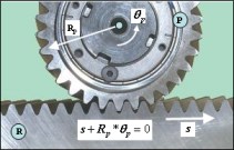
Figure 12 below depicts a rack and pinion joint.  The pinion gear P is connected to the housing (not shown) such that it is allowed to rotate about an axis coming out the plane of the paper.  The rack R slides from left-to-right.  The RACK_PINION joint relates the rotation of the pinion θp to the translation of the rack S.

Figure 12: A RACK_PINION joint

The RACK_PINION joint allows five degrees of freedom.  It imposes only one constraint on the system.

Figure 13 shows a schematic of a REVOLUTE joint.  This joint constrains two Reference_Markers I and J such that (a) their origins are always superposed, and (b) their z-axes are collinear.

Figure 13: A REVOLUTE joint

The REVOLUTE joint removes five degrees of freedom from a system. Rotation about the common z-axes is the only motion that is allowed.

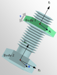
Figure 14 depicts a screw joint. Body-2 contains screw-threads with a pitch p. The axis of the screw is defined by the z-axis of a Reference_Marker J on Body-2. Body-1 has corresponding threads that allow it to mate with the threads on Body-2.  A rotation of Body-2 along the screw axis causes Body-1 to translate up or down along the screw axis. The SCREW joint relates the rotation of the Body-1 about the screw axis to its translation along the screw axis.

Figure 14: A SCREW joint

The SCREW joint removes only one degree of freedom from a system.

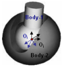
Figure 15 shows a schematic of a SPHERICAL joint. This joint constrains two Reference_Markers, I on Body-1 and J on Body-2, such that their origins Oi and Oj are always superposed.

Figure 15: A SPHERICAL joint

The SPHERICAL joint removes three degrees of freedom from a system. Body-2 is allowed to rotate with respect to Body-1. Relative translation is not allowed.

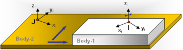
Figure 16 shows a schematic of a TRANSLATIONAL joint. This joint constrains two Reference_Markers I and J such that (a) their orientations remain the same, and (b) they share a single common axis of translation which is the z-axis of Reference_Marker J.

Figure 16: A TRANSLATIONAL joint

The TRANSLATIONAL joint removes five degrees of freedom from a system. Relative translation along the z-axis of Reference_Marker J is the only motion that is allowed.

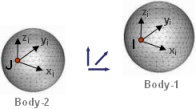
Figure 17 below shows a schematic of a UNIVERSAL joint. This joint constrains two Reference_Markers, I on Body-1 and J on Body-2 such that (a) their origins Oi and Oj remain superposed and (b) their z-axes are always orthogonal.

Figure 17: A UNIVERSAL joint

The UNIVERSAL joint removes four degrees of freedom from a system. Body-2 can rotate about the Zj axis and Body-1 can rotate about the Zi axis. Relative translations are not allowed.

Note that the output angular velocity will not be equal to the input angular velocity.

Let:

Then:

At β=π/2, the output angular velocity is zero.  Physically, the shafts lock.  This manifests itself as a singular matrix in MotionSolve.

Only at β=0, is the output shaft angular velocity equal to the input shaft angular velocity.

The angular acceleration of the output shaft, α2, can be expressed as:

Example

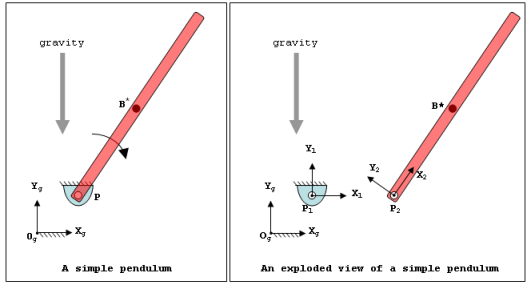
The image below shows a simple pendulum system.  The system consists of a rigid bar B that is pinned to Ground G at point P.  The center of mass of the Bar B is denoted by a Reference_Marker B*.

The connection at P requires that the corresponding material points on B (P1) and G (P2) always be superposed.  It also requires that the axis coming out of the plane of the paper at P1 and a second axis at P2 always remain collinear. This is a connection of type "REVOLUTE".

Gravity acts in the global negative Y direction.  Due to the effect of gravity, bar B swings in the global X-Y plane while satisfying the requirements that P1 and P2 remain superposed and the axes remain collinear.

A simple pendulum system illustrating the use of a REVOLUTE joint

If we define the following objects in the input data file:

The Constraint_Joint object may be defined as:

<Constraint_Joint

    id           = "1"

    label        = “Name of Joint”

    i_marker_id  = "21"

    j_marker_id  = "11"

    type         = "REVOLUTE"

/>

Model Element

Description

JOINT is used to specify an idealized connector between two bodies by defining a set of lower pair constraints. Physically, the joint consists of two mating surfaces that allow relative translational and/or rotational movement in certain specific directions only.  The surfaces are abstracted away, and the relationships are always expressed as a set of equations between points and directions on two bodies.

Declaration

def JOINT(id, LABEL="", I=0, J=0, TYPE="", PD=0.0, PITCH=0.0, IC=[], ICTRAN=[], ICROT=[]):

Attributes

id

Element identification number (integer>0).  This number is unique among all the JOINT elements.

LABEL

The name of the JOINT element.

I

Specifies the ID of the reference marker that defines the connection on the first body.  The body may be a rigid body, a flexible body, or a point body.  The parameter is required.

J

Specifies the ID of the reference marker that defines the connection on the second body.  The body may be a rigid body, a flexible body, or a point body.  The parameter is required.

TYPE

Specifies the type of constraint connection between the i_marker and j_marker_id.  The type can be one of the following:

"CONVEL"

"CYLINDRICAL"

"FIXED"

"HOOKE"

"PLANAR"

"RACKPIN"

"REVOLUTE"

"SCREW"

"SPHERICAL"

"TRANSLATIONAL"

"UNIVERSAL"

PD

Defines the pitch diameter of the pinion gear, a rack and pinion gear JOINT. The parameter is mandatory when TYPE ="RACKPIN"

PITCH

Defines the pitch of a screw JOINT.  The pitch defines the ratio between the translational and rotational motion in the screw joint.  The parameter is required only when TYPE = "SCREW".

IC

Specifies the initial velocity and initial displacement on either a translational or revolute joint.

ICTRAN

Specifies the initial translational velocity and initial translational displacement of the cylindrical joint.

ICROT

Specifies the initial rotational velocity and initial rotational displacement of the cylindrical joint.

Comments

See Constraint_Joint

Example

The example below shows a simple revolute joint between two bodies.

JOINT(1,LABEL="Name of the joint",I=21,J=11,TYPE="REVOLUTE")