|
»Click here to display Table of Contents«
|

Example 13 - Shock Tube |

|

|

|

|
|
Example 13 - Shock Tube |
|
|
|

|
|
»Click here to display Table of Contents«
|
Example 13 - Shock Tube |
|
|
|
|
|
Example 13 - Shock Tube |
|
|
|
|

This famous experiment is interesting for observing the shock-wave propagation. Moreover, this case uses the representation of perfect gas and compares the different formulations: The ALE uses Lagrangian or Eulerian and Smooth Particle Hydrodynamics (SPH).
The first part of the study deals with the modeling description of perfect gas with the hydrodynamic viscous fluid law 6. The purpose is to test the different formulations:
| • | Lagrangian (mesh points coincident to material points) |
| • | Eulerian (mesh points fixed) |
For the Eulerian formulation, different scale factors on time step are also tested. Furthermore, the SPH formulation is also tested; which does not use mesh, but rather particles distributed uniformly over the volume.
The propagation of the gas in the tube can be studied in an analytical manner. The gas is separated into different parts characterizing the expansion wave, the shock front and the contact surface. The simulation results are compared with the analytical solution for velocity, density and pressure.
TitleShock tube |
|
||||||||||
Number13.1 |
|||||||||||
Brief DescriptionThe transitory response of a perfect gas in a long tube separated into two parts using a diaphragm is studied. The problem is well-known as the Riemann problem. The numerical results based on the SPH method and the finite element method with the Lagrangian and Eulerian formulations, are compared to the analytical solution. |
|||||||||||
Keywords
|
|||||||||||
RADIOSS Options
|
|||||||||||
Compared to / Validation Method
|
|||||||||||
Input FileEulerian_formulation: <install_directory>/demos/hwsolvers/radioss/13_Shock_tube/Eulerian_formulation/TACEUL* Lagrangian_formulation: <install_directory>/demos/hwsolvers/radioss/13_Shock_tube/Lagrangian_formulation/TACLAG* SPH_hexagonal-net: <install_directory>/demos/hwsolvers/radioss/13_Shock_tube/SPH_formulation/TUBSPH* |
|||||||||||
Technical / Theoretical LevelAdvanced |
|||||||||||
The shock tube problem is one of the standard problems in gas dynamics. It is a very interesting test since the exact solution is known and can be compared with the simulation results. The Smooth Particle Hydrodynamics (SPH) method, as well as the Finite Element method using the Eulerian and Lagrangian formulations served in the numerical models.
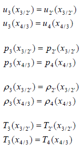
A shock tube consists of a long tube filled with the same gas in two different physical states. The tube is divided into two parts, separated by a diaphragm. The initial state is defined by the values for density, pressure and velocity, as shown in Figures 1 and 2. All the viscous effects are negligible along the tube sides; it is also assumed that there is no motion in the beginning.
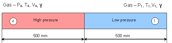
Fig 1: Sketch of the shock tube.
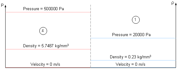
Fig 2: Initial states with discontinuities.
The initial state at time t = 0 consists of two constant states 1 and 4 with p4 > p1, ![]() 4 >
4 > ![]() 1, and V1 = V4 = 0 (table).
1, and V1 = V4 = 0 (table).
Table 1: Initial conditions in the shock tube.
|
High pressure side (4) |
Low pressure side (1) |
|---|---|---|
Pressure p |
500000 Pa |
20000 Pa |
Velocity u |
0 m/s |
0 m/s |
Density |
5.7487 kg/mm3 |
0.22995 kg/mm3 |
Temperature T |
303 K |
303 K |
Just after the membrane is removed, a compression shock runs into the low pressure region, while a rarefaction (decompression) wave moves into the high pressure part of the tube. Furthermore, a contact discontinuity usually occurs.
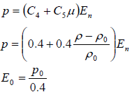
The hydrodynamic viscous fluid law 6 is used to describe compressed gas.
The general equation describing pressure is:
![]()
with ![]()
where, p is the pressure, Ci are the hydrodynamic constants, En is the internal energy per initial volume, and ![]() is the density.
is the density.
Perfect gas is modeled by setting all coefficients C0, C1, C2 and C3 to zero.
Also:
C4 = C5 = ![]() - 1
- 1
Where, ![]() is the gas constant.
is the gas constant.
Then the initial internal energy, per initial volume is calculated from initial pressure:
![]()
Under the assumption ![]() = CST = 1.4 (valid for low temperature range), the hydrodynamic constants C4 and C5 are equal to 0.4.
= CST = 1.4 (valid for low temperature range), the hydrodynamic constants C4 and C5 are equal to 0.4.
Gas pressure is described by:
Parameters of material law 6 are provided in Table 2.
Table 2: Material properties of gas in law 6.
|
High pressure side (4) |
Low pressure side (1) |
|---|---|---|
Initial volumetric energy density (E0) |
1.25x10⁶ J/m3 |
5x10⁴ J/m3 |
C4 and C5 |
0.4 |
0.4 |
Density |
5.7487 kg/mm3 |
0.22995 kg/mm3 |
The shock tube problem has an analytical solution of time before the shock hits the extremity of the tube [1].
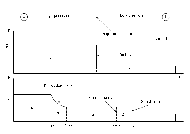
Fig 3: Schematic shock tube problem with pressure distribution for pre- and post-diaphragm removal.
Evolution of the flow pattern is illustrated in Fig 3. When the diaphragm bursts, discontinuity between the two initial states breaks into leftward and rightward moving waves, separated by a contact surface.
Each wave pattern is composed of a contact discontinuity in the middle and a shock or a rarefaction wave on the left and the right sides separating the uniform state solution. The shock wave moves at a supersonic speed into the low pressure side. A one-dimensional problem is considered.
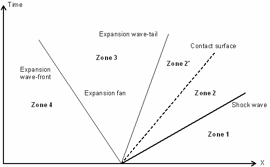
Fig 4: Diagram of the shock, expansion waves and contact surface.
There are four distinct zones marked 1, 2, 3 and 4 in Fig 4. Zone 1 is the low pressure gas which is not disturbed by the shock wave. Zone 2 (divided in 2 and 2' by the contact surface) contains the gas immediately behind the shock traveling at a constant speed. The contact surface across which the density and the temperature are discontinuous lies within this zone. The zone between the head and the tail of the expansion fan is noted as Zone 3. In this zone, the flow properties gradually change since the expansion process is isentropic. Zone 4 denotes the undisturbed high pressure gas.
Equations in Zone 2 are obtained using the normal shock relations. Pressure and the velocity are constant in Zones 2 and 2’.
The ratio of the specific heat constant of gas ![]() is fixed at 1.4. It is assumed that the value does not change under the temperature effect, which is valid for the low temperature range.
is fixed at 1.4. It is assumed that the value does not change under the temperature effect, which is valid for the low temperature range.
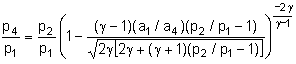
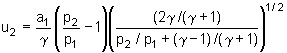
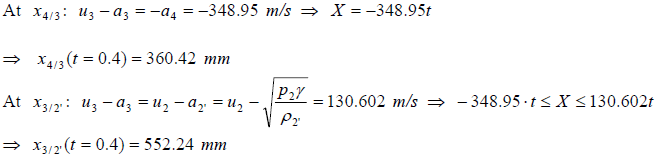
The analytical solution to the Riemann problem is indicated at t=0.4 ms. A solution is given according to the distinct zones and continuity must be checked. Evolution in Zones 2 and 3 is dependent on the constant conditions of Zone 1 and 4. The analytical equations use pressure, velocity, density, temperature, speed of sound through gas and a specific gas constant. Equations in Zone 2 are obtained using normal shock relations and the gas velocity in Zone 2 is constant throughout. The shock wave and the surface contact speeds make it possible to define the position of the zone limits.
|
Zone 4 |
Zone 1 |
|---|---|---|
Pressure p |
p4 = 500000 Pa |
p1 = 20000 Pa |
Velocity u |
u4 = 0 m/s |
u1 = 0 m/s |
Density |
|
|
Temperature T |
T4 = 303 K |
T1 = 303 K |
Speed of sound through gas:

Specific gas constant:

|
High pressure side (4) |
Low pressure side (1) |
|---|---|---|
a |
a4 = 348.95 m/s |
a1 = 348.95 m/s |
R |
287.049 J/(kg.K) |
|
|
Analytical solution |
Results at t = 0.4 ms |
|---|---|---|
Pressure p |
|
p2 = 80941.1 Pa |
Velocity u |
|
u2 = 399.628 m/s |
Density |
|
|
Temperature T |
|
T2 = 487.308 K |
Shock wave speed:
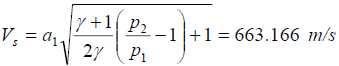
Therefore, x2/1 = Vs * 0.4 + 500 = 765.266 mm
|
Analytical solution |
Results at t = 0.4 ms |
|---|---|---|
Pressure p |
p2 = p2' |
p2' = 80941.1 Pa |
Velocity u |
u2 = u2' |
u2' = 399.628 m/s |
Density |
|
|
Temperature T |
p2' = r2'RT2' |
T2' = 180.096 K |
Surface contact speed: Vc - u2
Therefore, x2/2' = ![]() 2 * 0.4 + 500 = 559.85 mm
2 * 0.4 + 500 = 559.85 mm
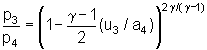
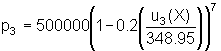
Zone 3 is defined as:
![]()
where, x = 500 + X
|
Analytical solution |
Results at t = 0.4 ms |
|---|---|---|
Pressure p |
|
|
Velocity u |
|
u3 = 290.792 + 2.0833 X |
Density |
|
|
Temperature T |
|
|
Continuity verifications:
Gas is modeled by 200 ALE bricks with solid property type 14 (general solid).
The model consists of regular mesh and elements, the size of which is 5 mm x 5 mm x 5 mm.
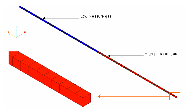
Fig 5: Mesh used for Lagrangian and Eulerian approaches.
In the Lagrangian formulation, the mesh points remain coincident with the material points and the elements deform with the material. Since element accuracy and time step degrade with element distortion, the quality of the results decreases in large deformations.
In the Eulerian formulation, the coordinates of the element nodes are fixed. The nodes remain coincident with special points. Since elements are not changed by the deformation material, no degradation in accuracy occurs in large deformations.
The Lagrangian approach provides more accurate results than the Eulerian approach, due to taking into account the solved equations number.
For the ALE boundary conditions (/ALE/BCS), constraints are applied on:
| • | Material velocity |
| • | Grid velocity |
The nodes on extremities have material velocities fixed in X and Z directions. The other nodes have material and velocities fixed in X, Y and Z directions.
The ALE materials have to be declared Eulerian or Lagrangian with /ALE/MAT.
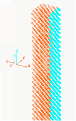
The 12798 particles are distributed though a hexagonal compact net. No mesh is used.
Fig 6: Smooth Particle Hydrodynamics modeling with hexagonal compact net.
The nominal value h0 is the distance between each particle and its closest neighbor. According to the assigned property of the part, the mass of the particles should be calculated. The mass is related to the density and the size of the net, in accordance with the following equation:
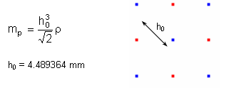
Where:
| • | Particle mass of low pressure part: mp = 1.25265x10⁻⁵ g |
| • | Particle mass of high pressure part: mp = 3.13166x10⁻⁴ g |
Particle mass is specified in the SPH property set.
The scale factor of the time step is set to 0.3 in order to ensure cell stability computation.
Boundary conditions are used to introduce SPH symmetry conditions (/SPHBCS). This option is specific to the SPH modeling and consists of creating ghost particles, symmetrical to the real particles with respect to the symmetry plane.
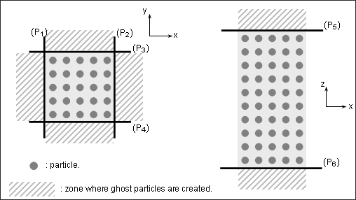
Fig 7: SPH symmetry planes definition.
Each symmetry condition is defined according to the plane passing through the frame origin attached to the plane and is normal in relation to the local direction of this frame.
Selected nodes and SPH symmetry condition frame along (-x) axis:
Six symmetry planes are used:
| • | x and (-x) symmetry conditions: SLIDE without rebound (Ilev =0) |
| • | y and (-y) symmetry conditions: SLIDE without rebound (Ilev =0) |
| • | z and (-z) symmetry conditions: TIED with elastic rebound (Ilev =1) |
For the SLIDE-type condition, the material is perfectly sliding along the plane
The particles must lie on the symmetry planes at t = 0.
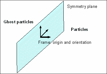
Fig 8: Local direction of frame
Particles should move into the positive semi-space defined as:
![]()
Where, O is the origin of the frame, P is a point of the plane, and ![]() is the local direction of the frame.
is the local direction of the frame.
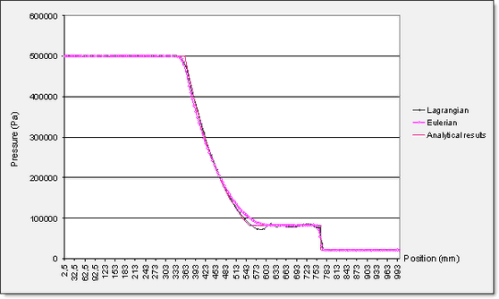
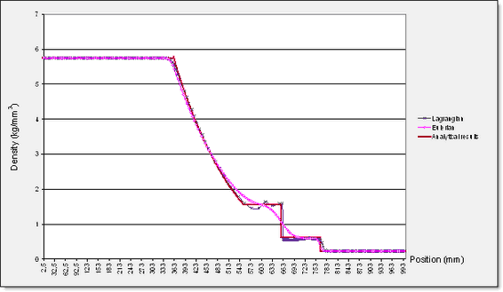
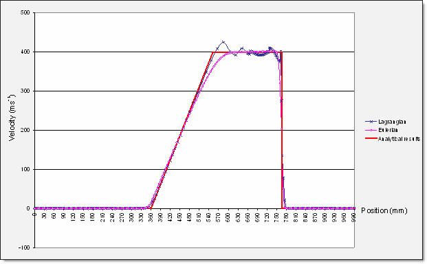
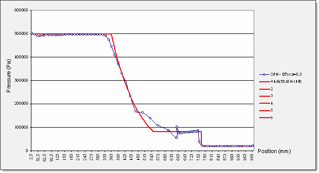
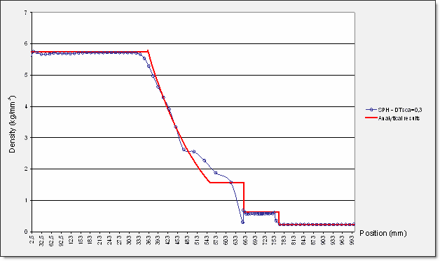
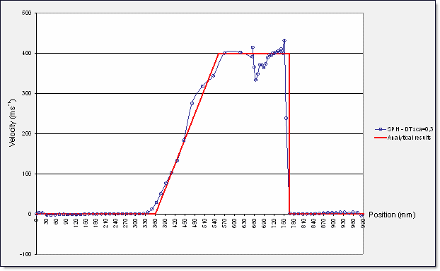
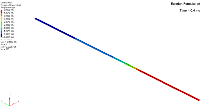
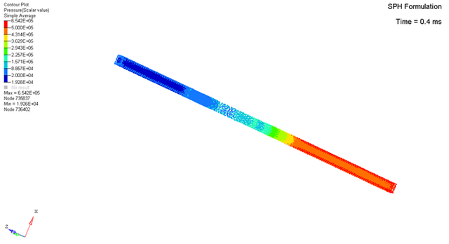
Simulation results along the tube axis at 0.4 ms are shown in the following diagrams.
Pressure |
|---|
|
Density |
|---|
|
Velocity |
|---|
|
| • | Lagrangian formulation: Scale factor = 0.1 |
| • | Eulerian formulation: Scale factor = 0.5 |
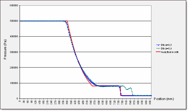
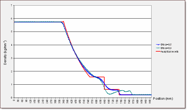
Case 1: Scale factor = 0.5
Case 2: Scale factor = 0.9
Pressure |
|---|
|
Density |
|---|
|
Simulation results along the tube axis at 0.4 ms. Scale factor: 0.3 and 0.67.
Pressure – Hexagonal Net and SPH Symmetry Conditions |
|---|
|
Density – Hexagonal Net and SPH Symmetry Conditions |
|---|
|
Velocity – Hexagonal Net and SPH Symmetry Conditions |
|---|
|
Indications on computation for each formulation are given in the following table (the scale factor is set to 0.5):
|
Finite Element approach |
SPH approach |
|
|---|---|---|---|
Formulation |
Lagrangian |
Eulerian |
SPH |
Normalized CPU |
1.08 |
1 |
1809 |
Number of cycles (normalized) up to 0.4 ms |
1.42 |
1 |
3.46 |
(DTsca=0.5)
|
|
|
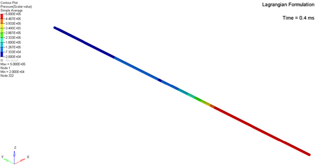
Fig 9: Pressure wave produced in the shock-tube at t = 4 ms for different approaches and animations regarding pressure, density and velocity
[1] J. D. Anderson Jr., Modern Compressible Flow with Historical Perspective, McGraw Hill Professional Publishing, 2nd ed., Oct. 1989.