Summary
The purpose of this example is to illustrate how to use the RADIOSS description when resolving a demonstration example. The particularities of the example can be summarized using dynamic loading during a four-step scenario where a dummy is first put on a bike, then it rides on a plane to subsequently jump back down onto the ground. The scenario described is created using sensors.
Title
Jumping bike
|
|
Number
12.1
|
Brief Description
After a quasi-static pre-loading using gravity, a dummy cyclist rides along a plane, then jumps down onto a lower plane. Sensors are used to simulate the scenario in terms of time.
|
Keywords
| • | Shell, brick, beam, truss, general spring, and beam |
| • | Sensors on rigid bodies and monitored volumes (perfect gas) |
| • | Quasi-static load treatment (gravity), kinetic relaxation, restart file, and MODIF file |
| • | Dummy and hierarchy organization |
| • | Type 7 interface self-impacting and rigid wall (infinite plane and parallelogram) |
|
RADIOSS Options
|
Input File
Jumping_bicycle: <install_directory>/demos/hwsolvers/radioss/12_Bicycle/Bike/BIKERC*
|
Technical / Theoretical Level
Advanced
|
Overview
Aim of the Problem
The purpose of this example is to set up a demonstration in which sensors and restart files are used to allow the change of a problem over time.
Physical Problem Description
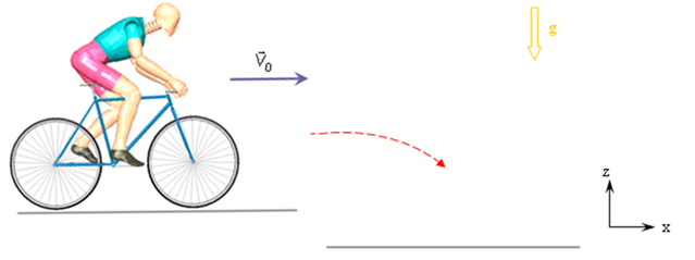
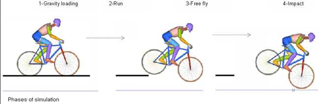
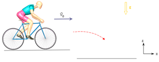
Subjected to the gravity field, a dummy cyclist rides on a higher plane, then jumps down onto a lower horizontal plane. The problem can be divided into four phases:
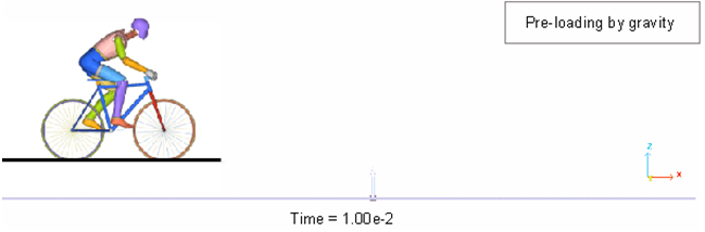
| • | positioning the cyclist under the gravity effect |
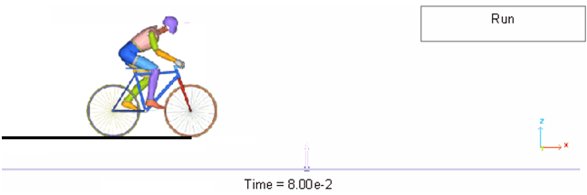
| • | running the bicycle on the high plane |
| • | the impact on the ground |
The following system is used: mm, s, ton, N, MPa
Fig 1: Problem scenario.
Analysis, Assumptions and Modeling Description
Modeling Methodology
The bike is meshed with 12103 4-node shells, 68 3-node shells, 62 trusses, 12 beams and six brick elements. The dummy consists of 4779 4-node shells, 207 3-node shell and 27 springs (8).
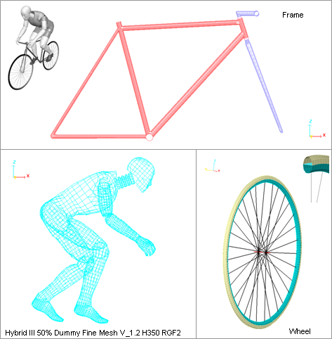
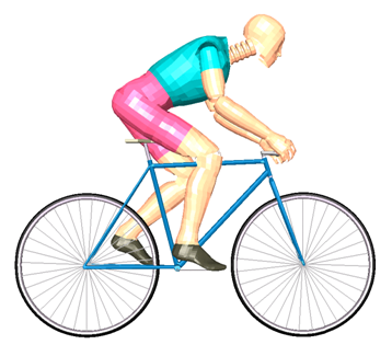
Fig 2: Meshes of the main parts of the model.
The material of the metallic parts use the Johnson-Cook law (/MAT/LAW2) with the following properties:
| • | Young’s modulus: 210000 MPa |
| • | Hardening parameter: 540 MPa |
| • | Hardening exponent: 0.32 |
A QEPH formulation (Ishell = 24) is used for tires in order to prevent hourglass deformations. A Belytschko & Tsay element with a type 4 hourglass formulation is used for the other shell parts. A global plasticity model is used.
Materials and proprieties are provided in the table below:
Table 1: Proprieties and materials of main parts
|
Parts
|
Properties
|
Materials
|
Bike
|
Frame
|
Shell Q4 – 3 mm
|
Steel – Law 2
|
Spokes
|
Truss – 2 mm2
|
Steel – Law 2
|
Rim
|
Shell Q4 – 3 mm
|
Steel – Law 2
|
Tires
|
Shell QEPH – 3 mm
|
Rubber – Law 1
|
Hubs
|
Beam – 900 mm2
|
Steel – Law 2
|
Saddle
|
Brick
|
Foam – Law 1
|
Pedals
|
Beam – 900 mm2
|
Steel – Law 2
|
Tube of saddle
|
Shell Q4 – 3 mm
|
Steel – Law 2
|
Dummy
|
Body (limbs)
|
Shell Q4 – 3 mm
|
Law 1
|
Joints
|
Spring (8)
|
-
|
Hierarchy organization:
| • | Bike model: 6 subsets comprising 23 parts |
| • | Dummy model: 11 subsets comprising 38 parts |
Monitored Volumes / Perfect Gas
A perfect gas monitored volume is defined to model the pressure in the tires. For further details about monitored volumes, refer to the RADIOSS Theory Manual.
The main properties are:
| • | External pressure: 0.1 MPa |
| • | Initial internal pressure: 0.75 MPa |
All other properties are set to default values.
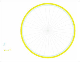
Fig 3: Visualization of a monitored volume (yellow part).
| • | Quasi-static loading: gravity effect on initial static equilibrium |
The quasi-static solution of gravity loading on structure deformation corresponds to the steady state part of the transient response. It describes the pre-loading case before the dynamic analysis. Therefore, the simulation is divided into two phases: quasi-static response (structure subjected to the gravity) and dynamic behavior (run, jump and landing). The solution is obtained from kinetic relaxation (see /KEREL). Gravity is defined by /GRAV.
The type 7 interface using the penalty method serves to model contacts between the dummy cyclist and the bike. An self-impacting interface (symmetrical) is required to treat the landing of the bike. It is modeled by a type 7 interface having default values. Figure 4 below illustrates the description of the interface.
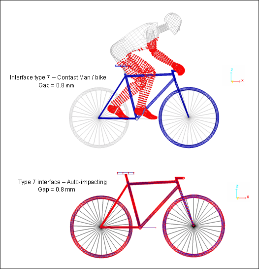
Fig 4: Contacts modeling with type 7 interface (Penalty method).
A type 11 interface models contact between the pedals (beams) and the feet (shells).
| • | Links between man and bicycle |
The spring type 8 (/PROP/SPR_GENE) general spring property model the links between the feet/pedals and the hands/handlebar.
| • | Stiffness (TX, TY and TZ): 100 kN/m |
A rupture criteria based on displacements is activated by the beams connecting the hands and handlebar in order to simulate the fall of the cyclist after landing.
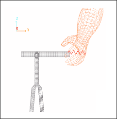
Fig 5: Link right hand/handlebar (Type 8 springs)
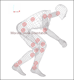
Fig 6: Type 8 Springs
The general type 8 springs, characterize a spherical hinge with a stiffness given for each DOF. Directions are local and attached to a moving skew frame. Two coinciding nodes define a spring.
Limbs are linked to the springs via the slave nodes of the rigid bodies, as shown in Fig 7.
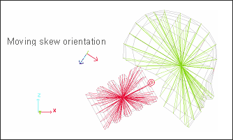
Fig 7: Example of connection rigid body – spring 8 – rigid body.
Beam elements are used to attach the wheel to the forks. The rotational DOF is released around the beam axis.
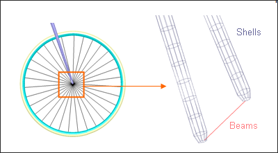
Fig 8: Wheel/forks junction
RADIOSS Options Used
Two types of rigid walls are set up:
| • | A fixed infinite plane (floor) |
| • | A fixed parallelogram (springboard) |
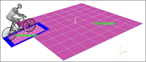
Fig 9: Position of the rigid walls
The characteristics of the parallelogram plane are: 2013 mm x 1200 mm. Both rigid walls are tied to allow the wheels to turn.
The infinite plane is defined by the normal vector ( ) and the parallelogram by the coordinates of three corners (M, M1, and M2). For both rigid walls, the slave nodes are obtained from the tire and rim parts (displayed in green in Fig 10).
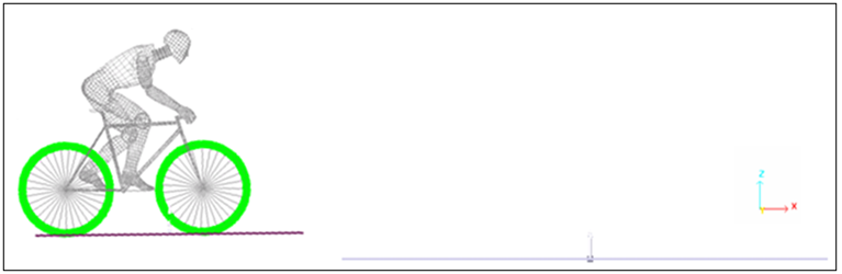
Fig 10: Slave nodes definition (green) and profile view of rigid walls
Several rigid bodies are created (/RBODY) and activated by sensors for use at the appropriate time and in a chronological manner (sens_ID not equal to 0). Thus, every rigid body is not active at the same time. The activation order is described in the paragraph dedicated to /SENSOR. According to their activation time, the rigid bodies are classified in groups which are indicated in following table.
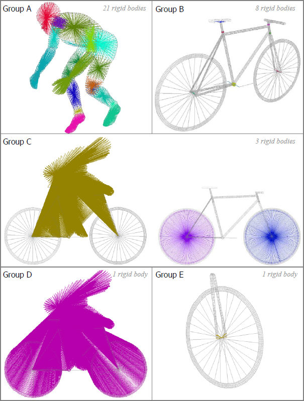
Fig 11: Classification of rigid bodies (group).
The inertias of rigid bodies are set in local skew frames for groups A, C and D.
Rigid body activation – deactivation:
Groups A and B: The rigid bodies are activated during pre-loading up to equilibrium then applied to the initial velocity start. They are activated again just before the impact of the bike on the inferior plane.
During the free fly phase, both the cyclist and the bike undergo a rigid body motion. In order to save the computation time, the motion can be simulated by putting the whole structure into a global rigid body (Group D). The rigid body is deactivated just before landing.
Group C: Three rigid bodies include the dummy, the frame and both wheels (not including the tires). This configuration allows just the wheels to turn, taking into account the active tires action on the plane. This rigid body is activated while the bike is running on the springboard.
Group D: This global rigid body, including all nodes of model is activated as long as the bike is in the free fly phase and is deactivated just before impact on the floor.
Group E: This rigid body is activated before impact ensures the stiffness level of the lower fork.
A 8333 mms-1 (30 km/h) initial velocity (/INIVEL) is applied to all nodes of the model (bicycle and cyclist) in a parallel direction to the high plane at time t = 0.004 s. This initial condition is defined in the Engine file “*_0002.rad" (start time: 0.004 s) which is run after the quasi-static equilibrium with gravity loading.
Options in Engine file (*_0002.rad):
/INIV/TRA/X/1  initial translational velocities in direction x
8333  of 8333 mm/s
1 338000 on node 1 to 338000
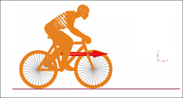
Fig 12: Initial translational velocities of the model bike – man (30 km/h) at t = 0.004 s.
Gravity is applied to all nodes of the model. A constant function defines the gravity acceleration in the Z direction versus time. Gravity is activated by /GRAV.
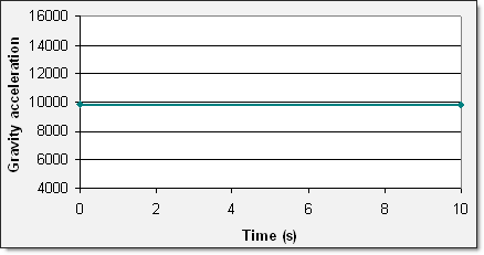
Fig 13: Gravity function (-9810 mm.s-2).
The explicit time integration scheme starts with the nodal acceleration computation. It is efficient for the simulation of dynamic loadings. Nevertheless, quasi-static simulations via a dynamic resolution method need to minimize the dynamic effects to converge towards the static equilibrium. Among the methods usually employed, the kinetic relaxation method is quite effective and is activated in the Engine file (*_0001.rad) with /KEREL. All velocities are set to zero each time the kinetic energy reaches a maximum value.
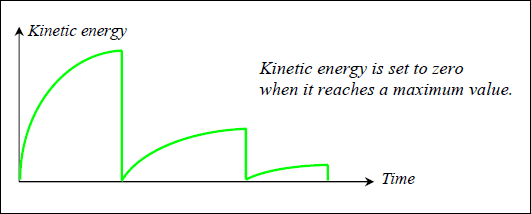
Fig 14: Kinetic relaxation method with /KEREL.
Rigid bodies are activated and deactivated with sensors (/SENSOR). A sens_ID flag characterizes the sensors and it is required in the rigid bodies’ definition. The five types of sensors used are:
| • | TIME (activated with time) |
| • | DIST (activated with nodal distance) |
| • | INTER (activated after impact on rigid wall) |
| • | SENSOR (activated with sensor IS1 and deactivated with sensor IS2) |
| • | NOT (ON as long as sensor IS1 is OFF) |
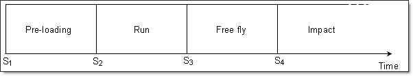
Fig 15: Events definition for the activations and deactivations of sensors.
At the beginning of the simulation (time=0), the rigid bodies are automatically set to ON, as long as the sensors are not active. Thus, in order to deactivate the rigid bodies at the first cycle, active sensors at time t=0 should be used. Consequently, the rigid bodies are active when the sensors are not active.
Added masses and inertia, as well as the flag for the gravity center, are ignored when a rigid body is managed by sensors. By default, the gravity center is only computed by taking into account the slave nodes mass (ICoG set at 2). The master node is moved to the computed center of gravity where added mass and inertia are placed. In order to distribute the mass to the dummy over the rigid bodies, option /ADMAS is used.
Sensors used are:
Table 2: Sensors used for simulation
Name
|
Type
|
Definition
|
Rigid body’s group using senor
|
S1
|
TIME
|
Time 0s.
|
-
|
S2
|
DIST
|
Distance between rear hubs and extremity of springboard equal to 1810 mm.
|
-
|
S3
|
DIST
|
Distance between rear hubs and extremity of springboard equal to 345 mm.
|
-
|
S4
|
RWALL
|
When the infinite rigid wall is impacted.
|
-
|
SEN(S2,S3)
|
SEN
|
Activated with S2 and deactivated with S3
|
-
|
SEN(S3,S4)
|
SEN
|
Activated with S3 and deactivated with S4
|
-
|
SEN(S2,S4)
|
SEN
|
Activated with S2 and deactivated with S4
|
Group A/B
|
NOT(SEN(S2,S3))
|
NOT
|
Deactivated with S2 and
activated with S3
|
Group C
|
NOT(SEN(S3,S4))
|
NOT
|
Deactivated with S3 and
activated with S4
|
Group D
|
Sensor (S4) is also used for deactivating both the beam type springs modeling links between the feet and pedals (Isflag set to 1). A case could be considered without this sensor to study the risks of automatic pedals.
The following graphs show the active and deactivated zones of sensors and rigid bodies.
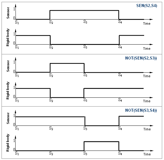
Fig 16: Activation and deactivation of sensors and rigid bodies.
Simulation Results and Conclusions
The elements included in a rigid body are deactivated. Therefore, the element flags saved in /TH/RBODY provide information on the activation and deactivation of rigid bodies during simulation.
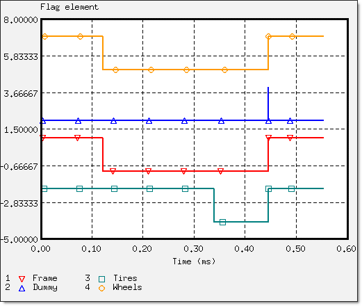
Fig 17: Activation and deactivation of main model parts (elements flag ON/OFF).
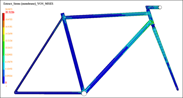
Fig 18: Distribution of the von Mises stress on the frame after quasi-static loading.
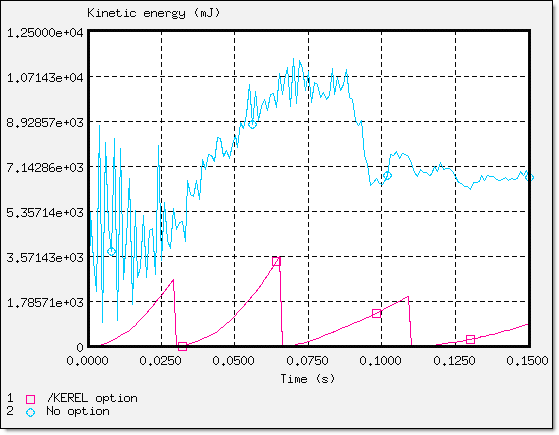
Fig 19: Kinetic relaxation effect on kinetic energy with /KEREL.
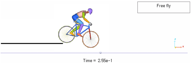
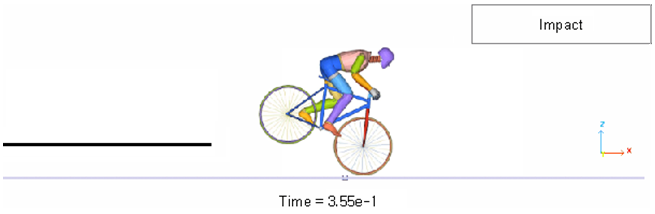
Fig 20: Simulation phases (impact at t = 4.6 s).
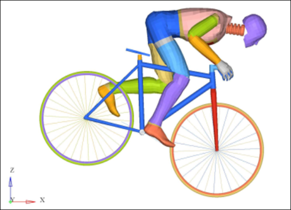
Fig 21: Configuration of a dummy cyclist during impact on the ground (shoes not attached).
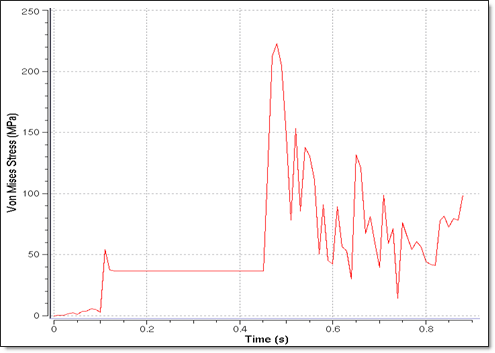
Fig 22: Variation of von Mises Stress for a shell element of the frame.