Summary
Elastic shock wave propagation on a half-space is studied using two different approaches:
| • | ALE (Arbitrary Lagrangian Eulerian) formulation |
The simulation results are compared with an analytical solution. A bi-dimensional problem is considered.
The domain subjected to the vertical impulse load undergoes an elastic material law process. The generated shock wave is composed of a longitudinal wave and a shear wave. Results are indicated in 0.77 ms, for which the longitudinal wave is predicted to reach the lower boundary of the domain. In order to ensure an accurate wave expansion, an infinite domain is modeled using a non-reflective frontiers (NRF) material law available in the ALE formulation.
Title
Lagrangian
|
|
Number
19.1
|
Brief Description
Elastic wave propagation on a half-space subjected to a vertically-distributed load.
|
Keywords
| • | Bi-dimensional analysis, quad and general solid |
| • | Impulse load, shock wave propagation, longitudinal and shear waves |
| • | ALE and Lagrangian modeling |
| • | Non-reflective frontiers (NRF) material and infinite domain |
|
RADIOSS Options
| • | Bi-dimensional analysis (/ANALY) |
| • | Non-reflective frontiers (NRF) material law 11 (/MAT/BOUND) |
|
Compared to / Validation Method
| • | Lagrangian vs. ALE modeling/Analytical solution |
|
Input File
Lagrangian modeling: <install_directory>/demos/hwsolvers/radioss/19_Wave_propagation/Lagrangian_formulation/WAVE*
ALE modeling: <install_directory>/demos/hwsolvers/radioss/19_Wave_propagation/ALE_formulation/WAVE*
|
Technical / Theoretical Level
Medium
|
Overview
Aim of the Problem
This example studies wave propagation through a bi-dimensional domain. Two analysis' are performed using:
| • | a Lagrangian formulation |
| • | an ALE (Arbitrary Langrangian Eulerian) formulation |
The simulation results are compared to an analytical solution.
Physical Problem Description
A half-space is subjected to a vertical load distributed over a varied time span and creating wave propagation in the domain. The dimensions of the model are 8 m x 4.76 m and the impulse load is applied over a 1 m-width zone.
Units: m, s, Kg, N, Pa.
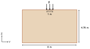
Fig 1: Problem data.
The material used follows a linear elastic law (/MAT/LAW1) and has the following characteristics:
| • | Initial density: 2842 kg.m-3 |
The expansion process of the shock wave is comprised of the longitudinal and shear waves.
Based on these material properties, the propagation speed of longitudinal waves in the material correspond to 6169.1 m.s-1 and 3107.5 m.s-1 for shear waves. Thus, the longitudinal waves should reach the lower boundary of the domain in about 0.77 ms.
The wave pattern caused by a distributed load is shown in Fig 2.
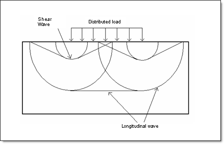
Fig 2: Longitudinal and shear waves comprising the wave pattern.
The impulse load is described by the sinusoidal function: F(t) = sin(2 * 105t) GPa
Analysis, Assumptions and Modeling Description
Modeling Methodology
The part is modeled using a regular mesh with 19080 QUAD elements (44.9 mm x 44.4 mm with lc =63.15 mm).
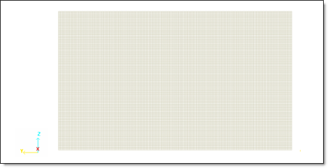
Fig 3: Mesh of the bi-dimensional domain.
RADIOSS Options Used
A bi-dimensional problem is considered. The flag N2D3D defined in /ANALY is set to 2. The 2D analysis defines the X-axis as the plane strain direction.
The applied vertical pulse is a concentrated load (/CLOAD) in the form of a sinusoidal function having an amplitude F = 1 GPa and a time period of T = 2 x E-5 s.
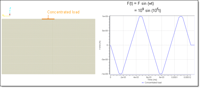
Fig 4: Variation of the impulse load over time.
Specific Options for the Lagrangian Modeling
Boundary conditions: Three sides of the model are fixed in terms of translation.
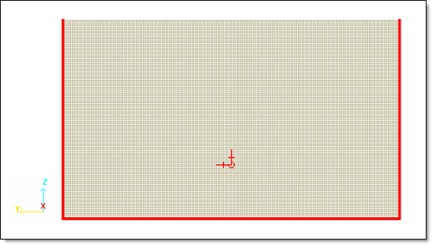
Fig 5: Fixed sides.
The limitation of this approach is the reflection on the domain’s boundaries. Simulation results are shown for the point in time prior to the shock hitting the low side (< 0.77 ms).
Specific Options for the ALE Modeling
Non-reflective frontiers (NRF): The mesh includes quiet boundary elements to model the infinite domain. These elements minimize the reflection of the propagating waves. The material used for these elements follow a non-reflective frontiers (NRF) material law 11 (type 3) as a non-reflective frontiers (NRF), and has the following characteristics:
| • | Initial density: 2842 kg.m3 |
| • | Characteristic length: 0.0632m |
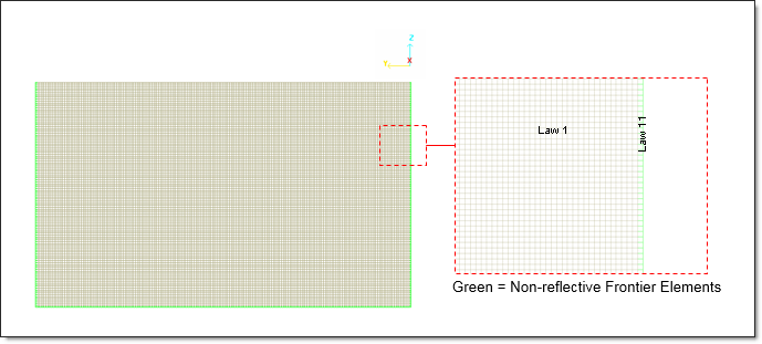
Fig 6: Infinite domain modeled by the non-reflective frontiers (NRF) material law 11 (type 3).
The materials have to be declared ALE using /ALE/MAT in the input desk.
Simulation Results and Conclusions
Comparison of Lagrangian and ALE Results with the Analytical Solution
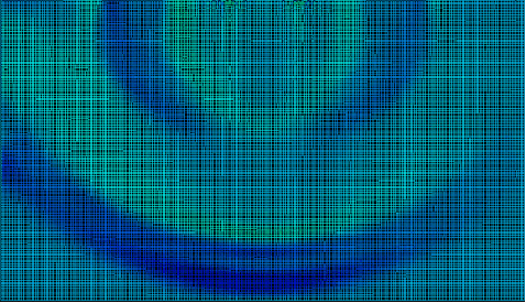
Figures 7 and 8 represent the von Mises stress wave propagation and the velocities at t=0.77 ms.
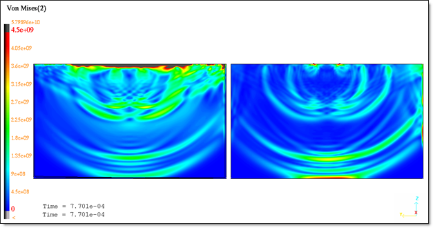
Fig 7: von Mises isovalues at t=0.77 ms.
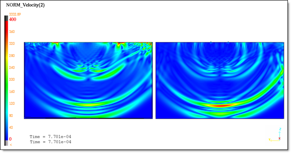
Fig 8: Velocity isovalues at t=0.77 ms.
The shock wave propagation is well predicted. Simulation results obtained at t=0.77ms corroborate the analytical solution: Longitudinal and shear waves.
Lagrangian Results
Wave Pattern
The wave pattern produced by the distributed load shown previously can be identified in the deformed configuration when the longitudinal wave reaches the lower boundary of the mesh.
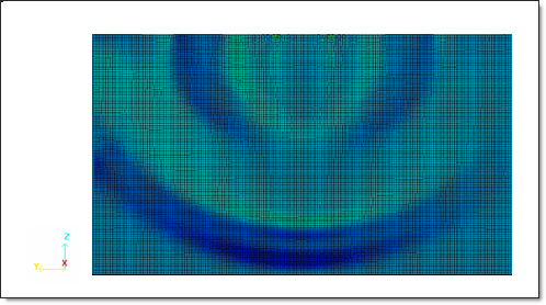
Fig 9: Wave pattern in domain at t=0.77 ms.
Vertical Displacement
The graphs below shows the vertical displacement (DZ) of three nodes respectively positioned at 0 m, 3.2 m and 4.75 m under the edge of the distributed load.
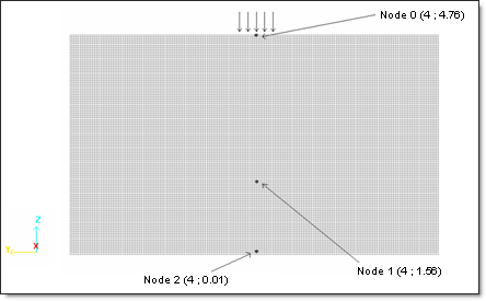
Fig 10: Nodes saved in Time History.
Figure 11 shows the vertical displacement of Node 0. The beginning of the wave propagation can be seen during the time [0; 1.35e-04]. The response after the end of the application force [1.35e-04; 4e-04] is due to the shear wave.
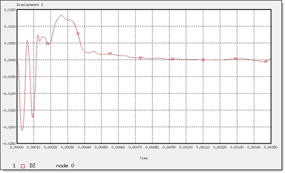
Fig 11: Z-displacement of "Node 0".
The vertical response of Node 1 shows that the longitudinal wave reaches it in 0.47 ms (Fig 12). The reflection can be seen after 0.97 ms. The shear wave does not appear because its motion is in the horizontal direction.
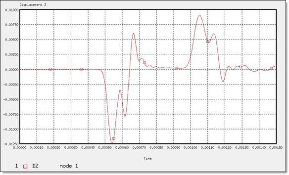
Fig 12: Z-displacement of "Node 1".
The displacement of Node 2 placed at the other extremity of the pattern, shows that the longitudinal wave crosses the model in 0.7 ms, in accordance with the analytical results.
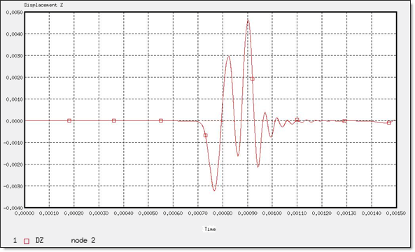
Fig 13: Z-displacement of "node 2".
Horizontal Displacement
Figure 14 shows the horizontal displacement of Node 1 (placed 3.2 m below the load surface). The horizontal component of the longitudinal wave reaches the node in 0.49 ms, while the shear wave arrives at 1.1 ms. Any response after this time results from the different reflections of the longitudinal and shear waves.
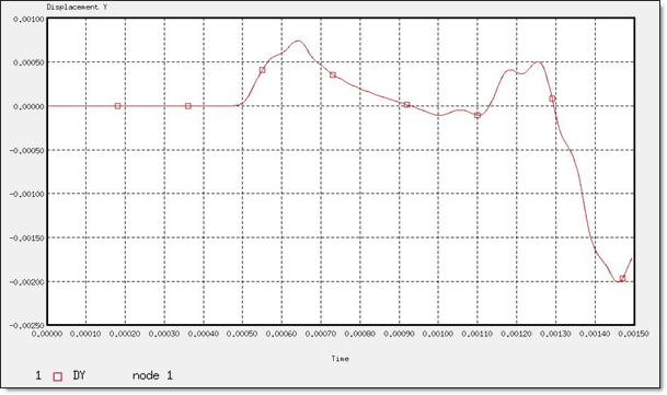
Fig 14: Y-displacement of "node 0".
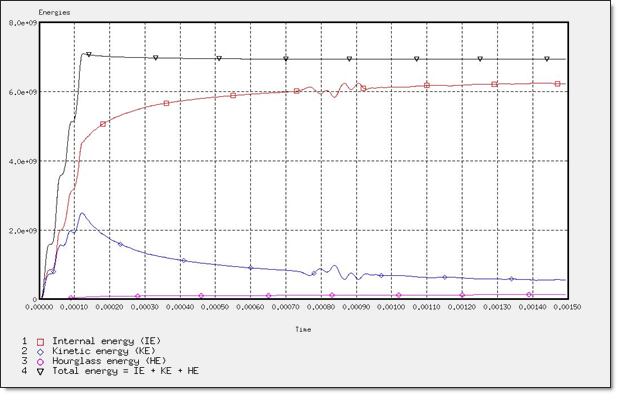
Fig 15: Global energy assessment.
ALE Results
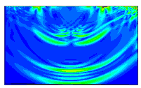
The wave pattern produced by a distributed load can be identified in the deformed configuration by displaying the pressure. The grid is fixed and nodal displacements are equal to zero. The following figure shows propagation when the longitudinal wave reaches the lower boundary of the mesh.
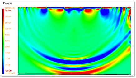
Fig 16: Pressure isovalues at time t=0.77 ms.
Conclusion
The wave propagation in a finite domain is studied using Lagrangian and ALE approaches. The Lagrangian formulation does not allow an infinite domain to be defined. Reflections of the longitudinal and shear waves against boundaries restrict simulation in terms of time (t < 0.77 ms). The ALE approach allows you to model an infinite domain by defining the non-reflective frontiers (NRF) material (Law 11 - type 3) on the limits. Such specific modeling minimizes the reflection of the expansion wave.
The bi-dimensional analysis illustrates a planar propagation. An accurate representation of the wave pattern is obtained and the simulation results are in a closed agreement with the analytical solution.


