
Summary
The fall of an ice cube dropping on two sloped beams is studied to illustrate the use of an explicit time integration scheme in resolving a transient dynamic analysis with free deformable flying objects. The impact and the rebound are modeled easily using various types of RADIOSS contact algorithms. Due to the rotary motion of the ice cube, a co-rotational solid formulation is required.
Title
Cube
|
|
Number
20.1
|
Brief Description
Ice cube dropping on two sliding channels.
|
Keywords
| • | Brick elements and 16-node shell elements |
| • | Co-rotational formulation |
|
RADIOSS Options
| • | Boundary conditions (/BCS) |
|
Input File
Model: <install_directory>/demos/hwsolvers/radioss/20_Cube/CUBE*
|
Technical / Theoretical Level
Beginner
|
Overview
Aim of the Problem
This problem demonstrates comparing two interfaces which will allow a sliding contact between an ice cube and the steel beams to be modeled.
Physical Problem Description
The cube is submitted to gravity and slides on inclined fixed beams and is collected in a cup. The width of the cube is 30 mm and the dimensions of the beams are 40 x 30 x 500 mm.
The material used for the cube is ice and has a linear elastic behavior (/MAT/LAW1), with the following characteristics:
| • | Initial density: 916 Kg/m3 |
| • | Young modulus: 10000 MPa |
The material used for the beams and the cup is steel and follows an isotropic elasto-plastic material (/MAT/LAW2) with the Johnson-Cook plasticity model, having the following characteristics:
| • | Initial density: 7800 kg/m3 |
| • | Young modulus: 210000 MPa |
| • | Hardening parameter: 450 MPa |
Units: m, s, Kg, N, Pa
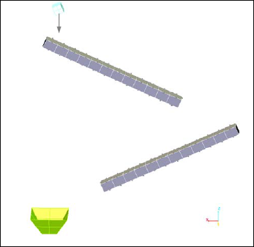
Fig 1: Overview of the problem.
Analysis, Assumptions and Modeling Description
Modeling Methodology
Contact between the ice cube and the first beam is modeled using a type 16 interface. Contact between the ice cube and the second beam is modeled using a type 7 interface. A type 7 interface defines contact between the ice cube and the cup.
| • | The first beam is modeled using twelve 16-node thick shell elements. |
| • | The second beam is modeled using twelve 8-node brick elements. |
| • | The ice cube is modeled using 8-node brick elements having a co-rotational solid formulation. |
| • | The cup is modeled with twelve standard shell elements. |
RADIOSS Options Used
Boundary conditions:
| • | The ice cube nodes are constrained in the Y translation and rotation is around the X-Z axis. |
| • | The lower nodes of the beams are constrained in all directions. |
| • | The cup is constrained in all directions. |
Load:
| • | A gravity load (g = 9.81 m/s2) in the Z-direction is applied on the ice cube’s nodes. |
Interface:
| • | The type 16 interface is used by deactivating the "tied" option, which enables a sliding contact to be modeled. Ice cube nodes are slave and the upper surface of the beam defines the master surface. |
| • | The type 7 interface between the ice cube and the second beam uses the Penalty method, with an initial gap of 1.5 mm. Ice cube nodes are slave and the master surface is defined using the upper surface of the beams. Friction is not taken into account. |
| • | The type 7 interface between the ice cube and the cup uses the same parameters as those defined above. Ice cube nodes are slave and the cup defines the master surface. |
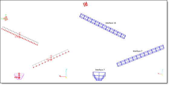
| Fig 2: Boundary conditions. | Interfaces. |
Simulation Results and Conclusions
The results below represent the trajectory of the ice cube and the cube’s reaction forces on the channels. The ice cube trajectory is obtained using a post-processing option, which enables to draw the trajectory of a picked node (here the center ice cube node) throughout simulation.
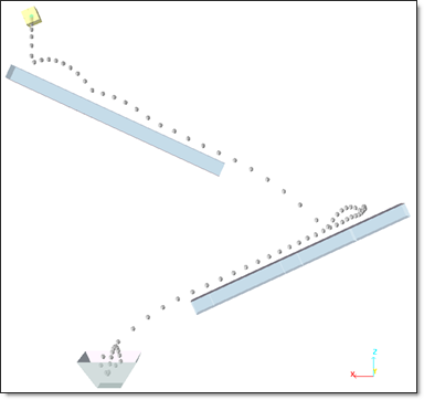
Fig 3: Trajectory of the ice cube.
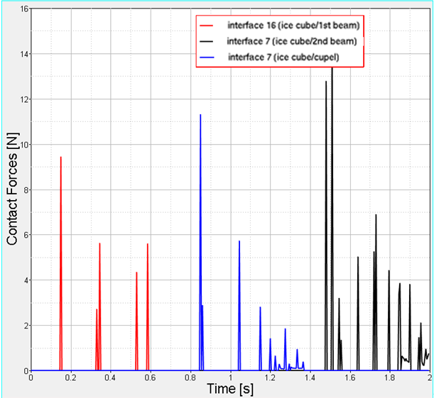
Fig 4: Reaction forces of the ice cube on channels.
Conclusion
This demonstrative example illustrated the capacity of RADIOSS to simulate sliding contacts, either using a Lagrangian (type 16 interface) or a Penalty method (type 7 interface).
The co-rotational solid formulation is essential in this case, taking into account the ice cube’s rotary motion.


