Summary
This example aims at demonstrating how to perform an FSI run using RADIOSS on a relatively simple case. The maximum deflection of a flap in an interaction with a transient fluid is computed once the stationary state is reached.
In this example, the two following points are emphasized:
| • | How to set up an FSI case study |
| • | Fast description of the various options used in an ALE/CFD run (refer to the RADIOSS Theory Manual for more information) |
Title
Biomedical Valve
|
|
Number
39.1
|
Brief Description
A Fluid-Structure-Interaction (FSI) problem is studied. The RADIOSS ALE/CFD solver is used to resolve the problem.
|
Keywords
|
RADIOSS Options
|
Input File
<install_directory>/demos/hwsolvers/radioss/39_Bio_Valve/BIO_VALVE/VALVE*
|
Technical / Theoretical Level
Skilled
|
Overview
Physical Problem Description
A simplified heart valve is modeled. The valve opens under the pressure of the incoming blood flow. As the opening process of the valve is taken into account, the problem is transient.
Additionally, fluid-structure interaction must be taken into account, as the flap deforms under the pressure of the blood.
Units: Kg, m, s, N, Pa
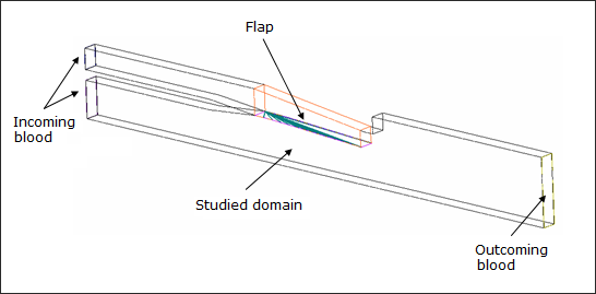
Fig 1: Definition of the problem.
RADIOSS ALE/CFD Terminology
Euler Formulation
The Eulerian formulation is classical in fluid mechanics. The mesh is fixed and material flows through the mesh. Equations are modified with respect to the Lagrangian formulation in order to take into account the convective terms.
It can be activated for a specific part by a flag in material data:
/EULER/MAT/mat_ID
Where, mat_ID is the identification number of the material to be set Eulerian.
In this case, the Eulerian formulation cannot be used because the boundaries of the domain (and mainly the flap) move.
ALE (Arbitrary Lagrangian Eulerian) Formulation
The material flows through an arbitrary moving mesh and it can degenerate either in a Lagrangian or an Eulerian formulation.
This option can be activated for a specific part by a flag in material data:
/ALE/MAT/mat_ID
Where, mat_ID is the identification number of the material to be set ALE.
Grid velocities and displacements are arbitrary.
In practice, built-in algorithms determine smooth grid deformation according to displacements of the ALE domain boundaries. Several algorithms are available (DONEA, SPRINGS, DISP, and ZERO), in this case, the DISP option is used: the velocity of a node is computed using the average velocities of the connected nodes.
Boundary nodes between ALE and Lagrangian materials must be set Lagrangian: grid and material velocities are equal. Boundary nodes between ALE and Eulerian materials with must have a fixed grid velocity.
Both conditions are set using the /ALE/BCS option.
We can also specify extended boundary conditions for ALE nodes (grid velocity components can be set to 0 or to the material velocity), or impose grid velocities or ALE links to any nodes in a similar manner to classical kinematic conditions.
Nodal Boundary Conditions
Kinematic constraints act on material velocities and accelerations. In RADIOSS CFD, a wide variety of such constraints can be defined. For fluid applications, options of interest are:
| • | fixed and full slip boundary conditions |
| • | imposed velocities (for example: imposed flux at inlet) |
| • | rigid links (temporarily adds during restarts) |
| • | rigid bodies to model rigid structures and connections and also to compute drag and lift forces (that is: fluid impulse on rigid body is stored in time history database) |
Grid constraints act only on grid velocities. You can specify:
| • | fixed and full slip grid conditions |
| • | Lagrangian conditions, that is: grid and material velocity are set equal. |
| • | ALE links to maintain regular distribution of nodes. |
| • | imposed grid velocities (for example: moving inlet and outlet) |
Elementary Boundary Conditions
Boundary elements allow prescription of element values at domain boundaries. They can be specified by assigning material law type 11 (or type 18 in purely thermal cases) to boundary elements. Those are quads in 2D and solids in 3D. For each variable P, rho, T, k, epsilon, internal energy, you can recommend:
| • | imposed varying conditions according to user function |
| • | smoothly varying predefined function |
Non-reflective frontiers (NRF) (material type 11, option 3) ensures free field impedance to pressure and velocity fields.
With RADIOSS ALE/CFD, any combination of the above options can be specified. On the counterpart, the closure of the various convection and diffusion equations has to be verified carefully by you.
Generally the following elementary boundary conditions are used:
| • | Inlet, flux is imposed using imposed velocities; density, energy, and turbulent energy (that is, k) are imposed as constants. Continuity is imposed for pressure (display purposes only) and for epsilon. Turbulent energy, rho k is set to zero for external flows and to 1.5*rho*(0.06 Vin)2 for internal flows. |
| • | Outlet, continuity for all variables except pressure, which is imposed. When using the NRF option, you need to provide a value for sound speed and a typical relaxation length, which must be greater than the biggest wave length of interest. |
| • | Sides, continuity for all variables with NRF option or slip conditions without boundary elements. |
If no element exists at boundary, continuity is assumed but kinematic conditions are necessary to disallow fluxes; otherwise, the convection equation is not closed and the program might diverge.
Analysis, Assumptions and Modeling Description
A quasi-uniform solid mesh is used for domain discretization. One element through the thickness with a fine enough mesh along the axis is used.
Shell elements are used to model the flap. The flap is clamped on one side and its nodes are attached by the springs to the clamp. One row of meshes are created at each extremity to define inlet and outlet.
The problem is incompressible; therefore, in order to increase the time step, the speed of the sound in the fluid has been arbitrarily reduced to 50 m/s.
When doing such an approximate, it must be verified that the velocity of the fluid is much lower than the modified speed of the sound.
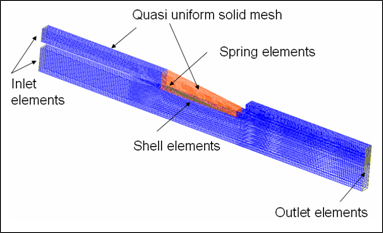
Fig 2: Mesh of the model
Four material laws are defined:
| • | A turbulent fluid material for the main parts of model (/MAT/LES_FLUID), |
/MAT/LES_FLUID
Rho = 960.0 Kg/m3
Sound speed = 50.0 m/s
Molecular kinematic viscosity = 5.45E-05 N.s/m
Sub-grid scale model flag = 0
Cs = 0.1
Csp = 0.1
| • | A fluid material for the inlet to define density, energy and pressure of fluid (/MAT/BOUND), |
/MAT/BOUND
Rho = 960.0 Kg/m3
Ityp = 2 (General case)
Sound speed = 50.0 m/s
| • | A fluid material for the outlet to define pressure of fluid outside the domain (/MAT/BOUND). |
/MAT/BOUND
Rho = 960.0 Kg/m3
Ityp = 3 Non-reflective frontiers (NRF)
Sound speed = 50.0 m/s
Characteristic length = 1.0E-03 m
The format /ALE/MAT is assigned to each of fluid materials.
Two imposed velocity are applied to the inlet nodes:
| • | Upper inlet: Vx= 1.253 m/s |
| • | Lower inlet: Vx= 0.849 m/s |
The boundary conditions are defined in the following table:
|
Type
|
Position
|
Boundary Condition
|
1
|
/BCS
|
Lateral nodes
|
Translation Vz = 0
|
2
|
/ALE/BCS
|
Lateral nodes
|
Grid velocity Wz = 0
|
3
|
/BCS
|
Nodes domain on the lateral edge of flap
|
Translation Vz = 0
|
4
|
/ALE/BCS
|
Nodes domain on the lateral edge of flap
|
Wx = Vx
Wy = Vy
Wz = Vz
|
5
|
/BCS
|
Nodes on flap
|
Translation Vz = 0
Rotation Wx = 0
Rotation Wy = 0
|
6
|
/ALE/BCS
|
Nodes on flap
|
Wx = Vx
Wy = Vy
Wz = Vz
|
An interface type 2 is created to connect the nodes of fluid domain on the lateral edge of flap, to the Lagrangian mesh of flap. Thus, the fluid domain is connected to the structural part.
With the use of this method, it is possible to have different meshes and mesh densities between the fluid and the structure.
Simulation Results and Conclusions
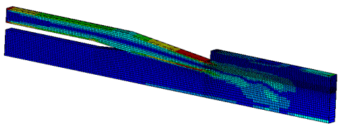
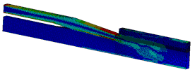
Vorticity distribution in the transient period gives a good overview of the problem evolution in time before stabilization.
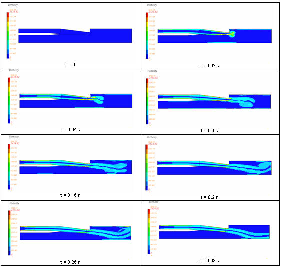
Fig 3: Vorticity distribution in time and in space
The main purpose of this study is to obtain the maximum deflection of the flap in time. Plotting the vertical displacement of the node 23360 given in the following graph in which the flap position is stabilized at time t=1 s.
The pressure stabilization in time is shown in Fig 5 for elements 3370 and 3992.
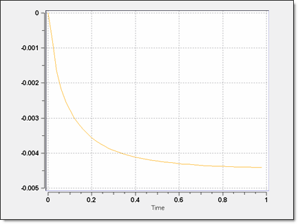
Fig 4: Vertical displacement of the free extremity (node 23360) of the flap in meter
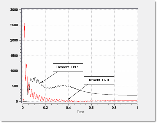
Fig 5: Pressure stabilization for elements 3370 and 3992 in Pa
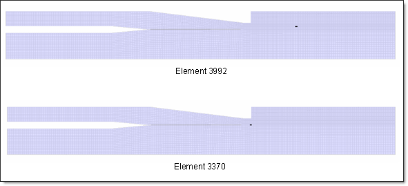
Fig 6: Position of elements 3992 and 3370
This example demonstrates RADIOSS capabilities to simulate transient Fluid-Structure-Interactions. The use of the ALE formulation attached to a Lagrangian mesh is described. Some elementary explanations to RADIOSS ALE/CFD terminology are mentioned.


