HyperWorks Solvers

Fatigue Analysis

Fatigue Analysis

Previous topic Next topic Expand/collapse all hidden text  

Fatigue Analysis

Previous topic Next topic JavaScript is required for expanding text JavaScript is required for the print function  

Introduction


Fatigue Analysis is intended for solutions to structures in a large number of loading cycles. Transient analysis is not effective in such cases since the elapsed time is generally very high and fatigue effects manifest over many loading cycles. In OptiStruct, both Uniaxial and Multiaxial Fatigue Analysis can be conducted.

hmtoggle_plus1Uniaxial Fatigue Analysis

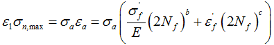
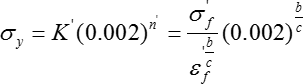
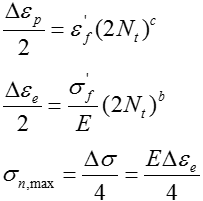
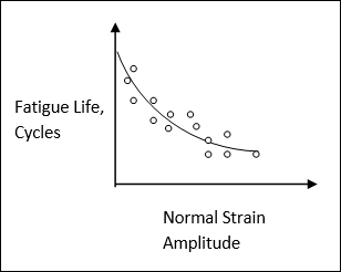
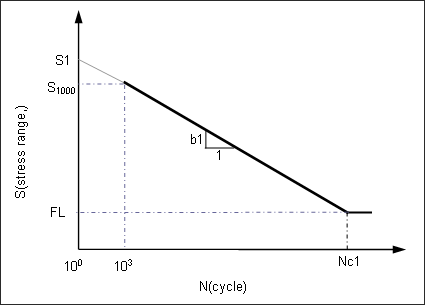
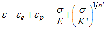
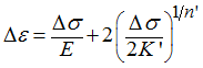
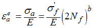
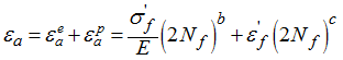
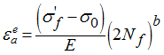
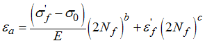
Uniaxial Fatigue Analysis, using S-N (stress-life) and E-N (strain-life) approaches for predicting the life (number of loading cycles) of a structure under cyclical loading may be performed by using OptiStruct.

The stress-life method works well in predicting fatigue life when the stress level in the structure falls mostly in the elastic range. Under such cyclical loading conditions, the structure typically can withstand a large number of loading cycles; this is known as high-cycle fatigue. When the cyclical strains extend into plastic strain range, the fatigue endurance of the structure typically decreases significantly; this is characterized as low-cycle fatigue. The generally accepted transition point between high-cycle and low-cycle fatigue is around 10,000 loading cycles. For low-cycle fatigue prediction, the strain-life (E-N) method is applied, with plastic strains being considered as an important factor in the damage calculation.

Sections of a model on which fatigue analysis is to be performed must be identified on a FATDEF Bulk Data entry. The appropriate FATDEF Bulk Data Entry may be referenced from a fatigue subcase definition through the FATDEF Subcase Information entry.

S-N Curve

The S-N curve, first developed by Wöhler, defines a relationship between stress and number of cycles to failure. Typically, the S-N curve (and other fatigue properties) of a material is obtained from experiment; through fully reversed rotating bending tests. Due to the large amount of scatter that usually accompanies test results, statistical characterization of the data should also be provided (certainty of survival is used to modify the S-N curve according to the standard error of the curve and a higher reliability level requires a larger certainty of survival).

fea_S-N_data2

Figure 1: S-N data from testing

When S-N testing data is presented in a log-log plot of alternating nominal stress amplitude Sa or range SR versus cycles to failure N, the relationship between S and N can be described by straight line segments. Normally, a one or two segment idealization is used.

fea_S-N_curves2

Figure 2: One segment S-N curves in log-log scale

for segment 1(1)

Where, S is the nominal stress range, Nf  are the fatigue cycles to failure, b1 is the first fatigue strength exponent, and S1 is the fatigue strength coefficient.

The S-N approach is based on elastic cyclic loading, inferring that the S-N curve should be confined, on the life axis, to numbers greater than 1000 cycles. This ensures that no significant plasticity is occurring. This is commonly referred to as high-cycle fatigue.

S-N curve data is provided for a given material on a MATFAT Bulk Data entry. It is referenced through a Material ID (MID) which is shared by a structural material definition.

Cycle Counting

Cycle counting is used to extract discrete simple "equivalent" constant amplitude cycles from a random loading sequence. One way to understand “cycle counting” is as a changing stress-strain versus time signal. Cycle counting will count the number of stress-strain hysteresis loops and keep track of their range/mean or maximum/minimum values.

Rainflow cycle counting is the most widely used cycle counting method. It requires that the stress time history be rearranged so that it contains only the peaks and valleys and it starts either with the highest peak or the lowest valley (whichever is greater in absolute magnitude). Then, three consecutive stress points (S1, S2, and S3) will define two consecutive ranges as symbol_triS1 = |S1 - S2| and symbol_triS2 = |S2 - S3|. A cycle from S1 to S2 is only extracted if symbol_triS1 symbol_lessthan symbol_triS2. Once a cycle is extracted, the two points forming the cycle are discarded and the remaining points are connected to each other. This procedure is repeated until the remaining data points are exhausted.

fea_rainflow_cycle

Figure 3: Determine cycles using rainflow cycle counting method

Parameters affecting rainflow cycle counting may be defined on a FATPARM Bulk Data entry. The appropriate FATPARM bulk data entry may be referenced from a fatigue subcase definition through the FATPARM Subcase Information entry.

Equivalent Nominal Stress

Since S-N theory deals with uniaxial stress, the stress components need to be resolved into one combined value for each calculation point, at each time step, and then used as equivalent nominal stress applied on the S-N curve.

Various stress combination types are available with the default being “Absolute maximum principle stress”. “Absolute maximum principle stress” is recommended for brittle materials, while “Signed von Mises stress” is recommended for ductile material. The sign on the signed parameters is taken from the sign of the Maximum Absolute Principal value.

Parameters affecting stress combination may be defined on a FATPARM Bulk Data entry. The appropriate FATPARM Bulk Data Entry may be referenced from a fatigue subcase definition through the FATPARM Subcase Information entry.

Damage Model (Mean Stress Influence)

Generally S-N curves are obtained from standard experiments with fully reversed cyclic loading. However, the real fatigue loading could not be fully reversed and the normal mean stresses have significant effect on fatigue performance of components. Tensile normal mean stresses are detrimental and compressive normal mean stresses are beneficial, in terms of fatigue strength. Mean stress correction is used to take into account the effect of non-zero mean stresses.

The Gerber parabola and the Goodman line in Haigh's coordinates are widely used when considering mean stress influence, and can be expressed as:

Gerber:

(2)

Goodman:

(3)

Where,

is the Mean stress given by

is the Stress Range given by

Se is the stress range for fully reversed loading that is equivalent to the load case with a stress range Sr and a mean stress

Su is the ultimate strength

The Gerber method treats positive and negative mean stress correction in the same way that mean stress always accelerates fatigue failure, while the Goodman method ignores the negative means stress. Both methods give conservative result for compressive means stress. The Goodman method is recommended for brittle material while the Gerber method is recommended for ductile material. For the Goodman method, if the tensile means stress is greater than UTS, the damage will be greater than 1.0. For the Gerber method, if the mean stress is greater than UTS, the damage will be greater than 1.0, with either tensile or compressive.

A Haigh diagram characterizes different combinations of stress amplitude and mean stress for a given number of cycles to failure.

haigh_diagram_11

Figure 4: Haigh diagram and mean stress correction methods

Parameters affecting mean stress influence may be defined on a FATPARM Bulk Data entry. The appropriate FATPARM bulk data entry may be referenced from a fatigue subcase definition through the FATPARM Subcase Information entry.

Damage Accumulation Model

Palmgren-Miner's linear damage summation rule is used. Failure is predicted when:

fatigue_eq(4)

Where, Nif is the materials fatigue life (number of cycles to failure) from its S-N curve at a combination of stress amplitude and means stress level i , ni is the number of stress cycles at load level i , and Di is the cumulative damage under ni load cycle.

The linear damage summation rule does not take into account the effect of the load sequence on the accumulation of damage, due to cyclic fatigue loading. However, it has been proved to work well for many applications.

Strain-life analysis is based on the fact that many critical locations such as notch roots have stress concentration, which will have obvious plastic deformation during the cyclic loading before fatigue failure. Thus, the elastic-plastic strain results are essential for performing strain-life analysis.

Neuber Correction

Neuber correction is the most popular practice to correct elastic analysis results into elastic-plastic results.

In order to derive the local stress from the nominal stress that is easier to obtain, the concentration factors are introduced such as the local stress concentration factor , and the local strain concentration factor .

(5)
(6)

Where, fea_symbol is the local stress, symbol_e is the local strain, S is the nominal stress, and e is the nominal strain. If nominal stress and local stress are both elastic, the local stress concentration factor is equal to the local strain concentration factor. However, if the plastic strain is present, the relationship between and no long holds. Thereafter, focusing on this situation, Neuber introduced a theoretically elastic stress concentration factor Kt defined as:

(7)

Substitute Eq.5 and Eq.6 into Eq.7, the theoretical stress concentration factor Kt can be rewritten as:

(8)

Through linear static FEA, the local stress instead of nominal stress is provided, which implies the effect of the geometry in Eq.8 is removed, thus you can set Kt as 1 and rewrite Eq.8 as:

(9)

Where, fea_symbole , Ee  is locally elastic stress and locally elastic strain obtained from elastic analysis, fea_symbol, symbol_e the stress and strain at the presence of plastic strain. Both fea_symbol and symbol_e can be calculated from Eq.9 together with the equations for the cyclic stress-strain curve and hysteresis loop.

Monotonic Stress-Strain Behavior

Relative to the current configuration, the true stress and strain relationship can be defined as:

(10)
fea_en_eq2(11)

Where, A is the current cross-section area, l  is the current objects length, l0 is the initial objects length, and fea_symbol and symbol_e are the true stress and strain, respectively, Figure 5 shows the monotonic stress-strain curve in true stress-strain space. In the whole process, the stress continues increasing to a large value until the object fails at C.

fea_monotonic_graph

Figure 5: Monotonic stress-strain curve

The curve in Figure 5 is comprised of two typical segments, namely the elastic segment OA and plastic segment AC. The segment OA keeps the linear relationship between stress and elastic strain following Hooke Law:

fea_segment_OA(12)

Where, E is elastic modulus and symbol_ee is elastic strain. The formula can also be rewritten as:

fea_seg_OA(13)

by expressing elastic strain in terms of stress. For most of materials, the relationship between the plastic strain and the stress can be represented by a simple power law of the form:

fea_power(14)

Where, symbol_ep is plastic strain, K is strength coefficient, and n is work hardening coefficient. Similarly, the plastic strain can be expressed in terms of stress as:

fea_stress_eq(15)

The total strain induced by loading the object up to point B or D is the sum of plastic strain and elastic strain:

fea_monotonic_eq(16)

Cyclic Stress-Strain Curve

Material exhibits different behavior under cyclic load compared with that of monotonic load. Generally, there are four kinds of response.

Stable state
Cyclically hardening
Cyclically softening
Softening or hardening depending on strain range

Which response will occur depends on its nature and initial condition of heat treatment. Figure 6 illustrates the effect of cyclic hardening and cyclic softening where the first two hysteresis loops of two different materials are plotted. In both cases, the strain is constrained to change in fixed range, while the stress is allowed to change arbitrarily. If the stress range increases relative to the former cycle under fixed strain range, as shown in the upper portion of Figure 6, it is called cyclic hardening; otherwise, it is called cyclic softening, as shown in the lower portion of Figure 6. Cyclic response of material can also be described by specifying the stress range and leaving strain unconstrained. If the strain range increases relative to the former cycle under fixed stress range, it is called cyclic softening; otherwise, it is called cyclic hardening. In fact, the cyclic behavior of material will reach a steady state after a short time which generally occupies less than 10 percent of the material total life. Through specifying different strain ranges, a series of hysteresis loops at steady state can be obtained. By placing these hysteresis loops in one coordinate system, as shown in Figure 7, the line connecting all the vertices of these hysteresis loops determine cyclic stress-strain curve which can be expressed in the similar form with monotonic stress-strain curve as:

fea_cyclic_resp2

Figure 6: Material cyclic response (a) Cyclic hardening; (b) Cyclic softening

fea_stable_curve

Figure 7: Definition of stable stress-strain curve

(17)

Where, K' is the cyclic strength coefficient and n' is the strain cyclic hardening exponent.

Hysteresis Loop Shape

Bauschinger observed that after the initial load had caused plastic strain, load reversal caused materials to exhibit anisotropic behavior. Based on experiment evidence, Massing put forward the hypothesis that a stress-strain hysteresis loop is geometrically similar to the cyclic stress strain curve, but with twice the magnitude. This implies that when the quantity fea_value is two times of fea_cycle, the stress-strain cycle will lie on the hysteresis loop. This can be expressed with formulas:

(18)
(19)

Expressing in terms of , symbol_e in terms of , and substituting it into Eq. 17, the hysteresis loop formula can be calculated as:

(20)

Almost a century ago, Basquin observed the linear relationship between stress and fatigue life in log scale when the stress is limited. He put forward the following fatigue formula controlled by stress:

(21)

Where, fea_symbola is the stress amplitude, fea_fatigue is the fatigue strength coefficient, and b is the fatigue strength exponent. Later in the 1950s, Coffin and Manson independently proposed that plastic strain may also be related with fatigue life by a simple power law:

(22)

Where, symbol_epa is the plastic strain amplitude, fea_fatigue2 is the fatigue ductility coefficient, and c is the fatigue ductility exponent. Morrow combined the work of Basquin, Coffin and Manson to consider both elastic strain and plastic strain contribution to the fatigue life. He found out that the total strain has more direct correlation with fatigue life. By applying Hooke Law, Basquin rule can be rewritten as:

(23)

Where, Eea is elastic strain amplitude. Total strain amplitude, which is the sum of the elastic strain and plastic stain, therefore, can be described by applying Basquin formula and Coffin-Manson formula:

(24)

Where, Ea is the total strain amplitude, the other variable is the same with above.

fea_strain-life_curve2

Figure 8: Strain-life curve in log scale

Damage Models (Mean Stress Influence)

The fatigue experiments carried out in the laboratory are always fully reversed, whereas in practice, the mean stress is inevitable, thus the fatigue law established by the fully reversed experiments must be corrected before applied to engineering problems.

Morrow

Morrow is the first to consider the effect of mean stress through introducing the mean stress fea_symbol0 in fatigue strength coefficient by:

(25)

Thus, the entire fatigue life formula becomes:

(26)

Morrow's equation is consistent with the observation that mean stress effects are significant at low value of plastic strain and of little effect at high plastic strain.

Smith, Watson and Topper

Smith, Watson and Topper proposed a different method to account for the effect of mean stress by considering the maximum stress during one cycle (for convenience, this method is called SWT in the following). In this case, the damage parameter is modified as the product of the maximum stress and strain amplitude in one cycle.

                 (27)

The SWT method will predict that no damage will occur when the maximum stress is zero or negative, which is not consistent with the reality.

When comparing the two methods, the SWT method predicted conservative life for loads predominantly tensile, whereas, the Morrow approach provides more realistic results when the load is predominantly compressive.

Damage Accumulation Model

In the E-N approach, use the same damage accumulation model as the S-N approach, which is Palmgren-Miner's linear damage summation rule.

hmtoggle_plus1Multiaxial Fatigue Analysis

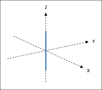
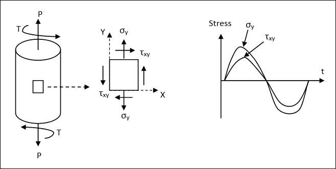
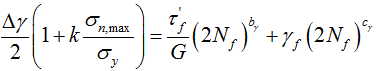
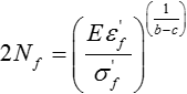
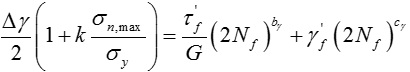
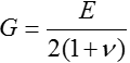
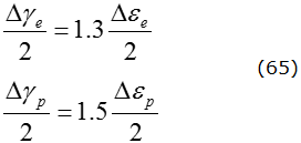
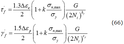
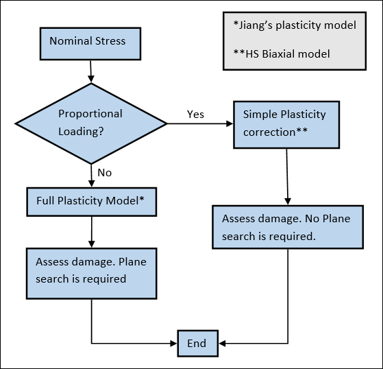
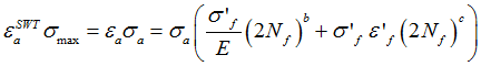
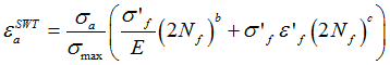
Multiaxial Fatigue Analysis, using S-N (stress-life), E-N (strain-life), and Dang Van Criterion (Factor of Safety) approaches for predicting the life (number of loading cycles) of a structure under cyclical loading may be performed by using OptiStruct.

In Uniaxial Fatigue Analysis, OptiStruct converts the stress tensor to a scalar value using user-defined combined stress method (von Mises, Maximum Principal Stress, and so on). In Multiaxial Fatigue Analysis, OptiStruct uses the stress tensor directly to calculate damage. Multiaxial Fatigue Analysis theories discussed in the following sections are based on the assumption that stress is in the plane-stress state. In other words, only free surfaces of structures are of interest in multiaxial fatigue analysis in OptiStruct. For solid elements, a shell skin is automatically generated by OptiStruct, shell elements are used as-is. Multiaxial Fatigue Analysis features are activated by setting MAXLFAT=YES on the FATPARM Bulk Data Entry.

The stress-life method works well in predicting fatigue life when the stress level in the structure falls mostly in the elastic range. Under such cyclical loading conditions, the structure typically can withstand a large number of loading cycles; this is known as high-cycle fatigue. When the cyclical strains extend into plastic strain range, the fatigue endurance of the structure typically decreases significantly; this is characterized as low-cycle fatigue. The generally accepted transition point between high-cycle and low-cycle fatigue is around 10,000 loading cycles. For low-cycle fatigue prediction, the strain-life (E-N) method is applied, with plastic strains being considered as an important factor in the damage calculation.

Sections of a model on which fatigue analysis is to be performed must be identified on a FATDEF Bulk Data Entry. The appropriate FATDEF bulk data entry may be referenced from a fatigue subcase definition through the FATDEF Subcase Information entry.

The Dang Van criterion is used to predict if a component will fail in its entire load history. The conventional fatigue result that specifies the minimum fatigue cycles to failure is not applicable in such cases. It is necessary to consider if any fatigue damage will occur during the entire load history of the component. If damage does occur, the component cannot experience infinite life.

Uniaxial Load

Models with uniaxial loads consist of loading in only one direction and result in one principal stress.

fatigue_uniaxial_load

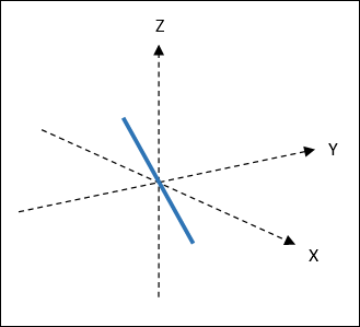
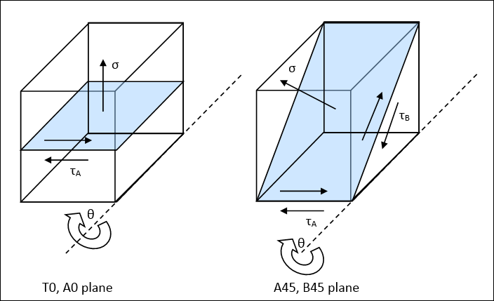
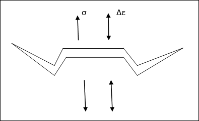
Figure 9: Uniaxial load

Proportional Biaxial Load

In models with proportional biaxial loads, principal stresses vary proportionally; however, still in one direction. Typically, in-phase loading of stress components is known as proportional biaxial load. Therefore, a fatigue subcase where a single static subcase is referenced is always a proportional biaxial load.

fatigue_biaxial_load

Figure 10: Proportional biaxial load

fatigue_biaxial_load2

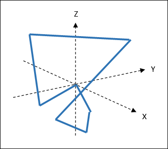
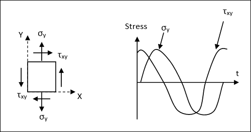
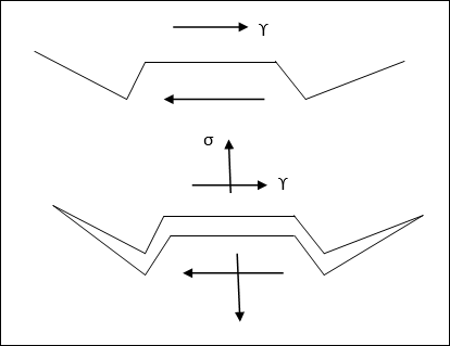
Figure 11: In-Phase load

In models with non-proportional biaxial loads, principal stresses can vary non-proportionally, and/or with changes in direction. Typically, out-of-phase loading of stress components is known as non-proportional multiaxial load.

Non-Proportional Multiaxial Load

fatigue_non-prop_multiaxial_load

Figure 12: Non-proportional multiaxial load

fatigue_non-prop_multiaxial_load2

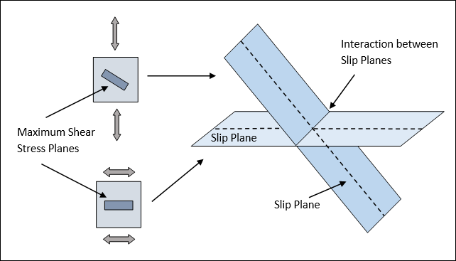
Figure 13: Out-of-Phase load

In Multiaxial Fatigue Analysis, proportional biaxial loads and non-proportional multiaxial loads are considered in OptiStruct.

Non-proportional Cyclic Loading and Non-proportional Hardening

Non-proportional cyclic loads typically generate additional strain hardening, which is not observed in the proportional loading environment. The additional strain hardening is called non-proportional hardening and is caused by interaction of slip planes. As a result of the rotation of the principal axes (Figure 12), multiple sliding planes are active, and hardening can accumulate at a certain point, while the direction of the slip plane changes.

fatigue_cyclic_non-prop_hardening

Figure 14: Interaction between slip planes, due to non-proportional loading.

The plasticity model used in multiaxial fatigue analysis will take care of non-proportional hardening, if applied load is non-proportional.

Experiments show that cracks nucleate and grow on specific planes known as critical planes. The Critical Plane Approach captures the physical nature of damage in its damage assessment process. It deals with stresses and strains on the critical planes. Depending on the material and stress states, the critical planes can be either maximum shear planes or maximum tensile stress planes. Therefore, in order to assess damage from multiaxial loads, two separate damage models are required. One is for crack growth due to shear, and the other is for crack growth due to tension.

fatigue_critical_plane_approach

Figure 15: Cracks driven by shear and tensile stress

fatigue_cracks

Figure 16: Cyclic Torsion, Shear Strain, Tensile Strain, Shear and Tensile Damage.

Any damage model can be used in the critical plane approach. The damage models require a search for the most damaging plane. There are two possible damaging (or failure) modes. One on planes that are perpendicular to the free surface which is tensile crack growth. The angle θ is the angle that a crack is observed on the surface relative to the σx direction. The second failure system occurs on planes oriented 45 degrees to the surface, which is shear crack growth. Both in-plane and out-of-plane shear stresses are considered on this plane. θ can take on any value on the surface. The shear stress symbol_tA is an in-plane shear stress and causes microcracks to grow along the surface. The maximum out-of-plane shear, symbol_tB occurs on a plane that is oriented at 45 degrees from the free surface and causes microcracks to grow into the surface.

fatigue_cracks2

Figure 17: In–plane shear stress and normal stress at 90 degree plane; in-plane and out-of-plane shear stress at a 45 degree plane.

OptiStruct searches for the most damaging plane by 10 degrees of θ. On each plane, OptiStruct assesses damage using tensile crack damage model and shear crack damage model. At the end of a search, OptiStruct reports damage at the most damaging plane which is a critical plane.

The Stress-Life Approach for the Multiaxial Fatigue Analysis is similar to Uniaxial Fatigue Analysis. See the S-N Curve and Cycle Counting sections of Uniaxial Fatigue Analysis for introductory information for Stress-Life approach in Multiaxial Fatigue Analysis.

Damage models

Depending on the material, stress state, environment, and strain amplitude, fatigue life will usually be dominated either by microcrack growth along shear planes or along tensile planes. Critical plane models incorporate the dominant parameters governing either type of crack growth. Due to the different possible failure modes, shear or tensile dominant, no single damage model should be expected to correlate test data for all materials in all life regimes. There is no consensus yet as to the best damage model to use for multiaxial fatigue life estimates. Multiple models are used in OptiStruct multiaxial fatigue analysis. For stress-based damage model, Goodman model is used for tensile crack. Findley model is used for shear crack. You can define damage models after the MDMGMDL field on the FATPARM Bulk Data Entry. If multiple damage models are defined, OptiStruct selects the worst damage model from all the available damages.

Goodman model

The Goodman model in uniaxial fatigue analysis is used at critical plane to assess damage caused by tensile crack growth.

Findley model

The Findley criterion is often applied for finite long-life fatigue.

fatigue_findley_eq      (28)

Where, fatigue_findley_symbol is computed from the torsional fatigue strength coefficient, fatigue_findley_symbol3, using:

fatigue_findley_eq2            (29)

The correction factor fatigue_findley_symbol2 typically has a value of about 1.04. Note that fatigue_findley_symbol has to be defined based on amplitude. If fatigue_findley_symbol3 is not defined by you, OptiStruct automatically calculates it using the following equation.

fatigue_eq2

The constant k is determined experimentally by performing fatigue tests involving two or more stress states. For ductile materials, k typically varies between 0.2 and 0.3. Its default value in OptiStruct is 0.3.

If CHK is set to YES in FATPARM for the proportional loadcase, the above equation is calculated on maximum shear stress plane. For more details, see Proportional Biaxial Load.

fatigue_flow_stress

Figure 18: Analysis flow for stress based multiaxial fatigue analysis

If the applied load is non-proportional multiaxial cyclic, OptiStruct runs the Jiang-Sehitoglu plasticity model to calculate the total strain and elasto-plastic stress. The Jiang-Sehitoglu model is one of the more successful incremental multiaxial cyclic plasticity models (Jiang and Sehitoglu "Modeling of Cyclic Ratcheting Plasticity, Part I: Development of Constitutive Equations," Journal of Applied Mechanics, Vol. 63, 1996, 720-725). In OptiStruct, isotropic hardening part is removed from Jiang-Sehitoglu's original model, which is best described in deviatoric stress space.

fatigue_plasticity_eq     (31)

Yield function

The Mises yield function, F, is expressed as:

fatigue_yield_function    (32)

The notation symbol_s_notion is used for the deviatoric stress tensor, symbol_a_backstress is the backstress tensor and k is the yield stress is simple shear.

Flow rule

The normality rule is given by:

fatigue_normality_rule_eq    (33)

Where, fatigue_exterior_unit_symbol is the exterior unit normal to the yield surface at the loading point, as defined below:

fatigue_flow_rule_eq       (34)

Hardening rule

The total backstress fatigue_total_backstress_symbol is divided into M parts.

fatigue_hardening_rule                    (35)

The evolution of the backstress (translation of the yield surface) for each of the parts is given by:

fatigue_backstress_evolution_eq    (36)

Where, dp is the equivalent plastic strain increment and ci, ri, and Xi are three sets of non-negative and single valued scalar functions:

fatigue_scalar_functions

Material memory is contained in the α terms. The plastic modulus function, H, is derived from the consistency condition which requires that the stress state be on the yield surface when plastic deformation is occurring.

fatigue_plastic_modulus_function     (40)

There are four material parameters in this model, c, r, X, and k. All of these constants are computed from the cyclic stress strain curve of the material (Eq. 17). A simple power function is fit to this curve to obtain three material properties; cyclic strength coefficient, K', cyclic strain hardening exponent, n', and elastic modulus, E.

The shear yield strength, k, is obtained by setting the plastic strain to 0.0002 (0.02%) and dividing by fatigue_square_root3 . Both c and r are obtained by selecting a series of stress strain pairs along the material cyclic stress strain curve and describe the shape of the curve. Ratcheting rate is controlled by X which is set at a fixed value of 5. The number of components (M) is set to 10.

Non-proportional Hardening

Non-proportional hardening is the term used to describe loading paths where the principal strain axes rotate during cyclic loading. The simplest example is a bar subjected to alternating cycles of tension and torsion loading. Between the tension and torsion cycles the principal axis rotates 45 degrees. Out-of-phase loading is a special case of non-proportional loading and is used to denote cyclic loading histories with sinusoidal or triangular waveforms and a phase difference between the loads. Materials show additional cyclic hardening during this type of loading that is not found in uniaxial or any proportional loading path.

The 90 degrees out-of-phase loading path has been found to produce the largest degree of non-proportional hardening. The magnitude of the additional hardening observed for this loading path as compared to that observed in uniaxial or proportional loading is highly dependent on the microstructure and the ease with which slip systems develop in a material. A non-proportional hardening coefficient, a, can be introduced which is defined as the ratio of equivalent stress under 90 degrees out-of-phase loading/equivalent stress under proportional loading at high plastic strains in the flat portion of the stress-strain curve. This term reflects the maximum degree of additional hardening that might occur for a given material. OptiStruct measures the non-proportional hardening coefficient, a, at 0.003 strain amplitude using:

fatigue_nonprop_hardening_coeffecient             (41)

Where,

fatigue_hardening_coefficient

You will need to input the coefkp90 and coefnp90. The default value of coefkp90 is 1.2. Default value of coefnp90 is 1.0.

The degree of non-proportionality, C, is a fourth ranked tensor which is a function of the plastic strain and the direction of the plastic strain increment.

fatigue_plastic_strain_increment    (42)

The amount of non-proportional hardening is computed from Tanaka's parameter. (Tanaka, E., "A Non-proportionality Parameter and a Cyclic Viscoplastic Constitutive Model Taking into Account Amplitude Dependencies and Memory Effects of Isotropic Hardening," European Journal of Mechanics, A/Solids, Vol. 13, 1994, 155-173).

fatigue_non-prop_hardening_eq         (43)

For any proportional loading A=0 and for 90 degrees out-of-phase loading A = 1/sqrt(2). The material constants, ri and the yield stress k are related to the non-proportional hardening parameter as follows:

fatigue_non-prop_hardening_parameters

The rate of hardening is controlled by the constant b. Since you are interested in the stable solution for fatigue calculations, b = 5 is selected for numerical stability. These equations are now sufficient to solve for the stresses and strains under any arbitrary loading path. The solution now proceeds by incrementally solving these equations, which can be solved in either stress, or strain control. The initial conditions are that the stress and backstress start at. All material constants start at their initial values as well and are updated after each loading increment.

Notch Correction

In uniaxial loading approximate solutions such as Neuber's rule are used to compute the stresses and strains during plastic deformation. Unfortunately, Neuber's rule cannot be directly extended to multiaxial loading because there are six unknowns and only five equations. To overcome this problem Koettgen (Koettgen V.B., Barkey M.E., and Socie, D.F. "Pseudo Stress and Pseudo Strain Based Approaches to Multiaxial Notch Analysis" Fatigue and Fracture of Engineering Materials and Structures, Vol. 18, No. 9, 1995, 981-1006) proposed a structural yield surface to obtain local elastic-plastic stresses and strains. Having defined a "yield surface," standard cyclic plasticity methods can be used to solve the unknown stresses and strains at the notch. The material memory effects are built directly into standard cyclic plasticity calculations. The method is based on the same concept at the analytical or experimental nominal stress - notch strain curves used in uniaxial fatigue analysis such as the one shown below.

Cyclically, nominal stress - notch root strain response has all the features associated with stress-strain response such as hysteresis, memory, cyclic hardening and softening. The concept of pseudo stress, fatigue_symbol3, or strain, fatigue_symbol4 , is defined as theoretical elastic stress or strain computed using elastic assumptions. Neuber's rule may be written in terms of pseudo stress as:

                (45)

These concepts can be generalized to three dimensional stress and strain states with a structural yield surface at a notch. Having defined a structural yield surface, standard cyclic plasticity methods can be used to solve the unknown stresses and strains at the notch. For multiaxial loading, the total stress or strain is obtained by superposition of the individual load cases. A relationship between pseudo stress and notch strain is described with a power function that has the same form as a stress-strain curve.

fatigue_stress_strain_curve            (46)

Where, the constants K* and n* represent the behavior of the structure rather than the material. Uniaxial Neuber's rule is employed to establish the constants E*, K* and n*.

For plane stress on the surface, fatigue_symbol5, fatigue_symbol6 and fatigue_symbol7 are all zero and this yield function can be written as:

       (47)

This equation defines a structural yield function, Fo, which has the same form as the yield functions used in the plasticity models for stress-strain calculations, i.e. a Mises yield function in terms of pseudo stress.

fatigue_structural_yield_function_eq        (48)

The process to calculate stress from pseudo stress is summarized as follows:

1.Apply uniaxial Neuber's rule to get K* and n* (Eq. 46).
2.Run Jiang-Sehitoglu plasticity model in pseudo stress control with pseudo constants K* and n* to obtain the pseudo stress-local strain response. Now total strain is available.

3.Run Jiang-Sehitoglu plasticity model in strain control with material constants K and n to obtain the local strain - local stress response. Finally stress is also available.

Proportional Biaxial Load

If applied load is proportional biaxial load, you do not have to calculate incremental plastic stress and strain using Jiang-Sehitoglu plasticity model. Because direction of principal stresses do not change, you know where the maximum shear stress and the maximum tensile stress are developed and what their values are with Mohr's circle. What you need to do is convert pseudo stress range to stress range using notch correction method such as Neuber's rule or Glinka's rule. OptiStruct applies Hoffmann-Seeger method for this situation.

If only one static subcase is referenced in FATEVNT, the cyclic load is always proportional biaxial load. In this case, if CHK is set to YES in FATPARM, OptiStruct runs Hoffmann-Seeger method to calculate stress and strain from pseudo stress. If multiple static subcases are referenced in FATEVNT, currently OptiStruct runs Jiang-Sehitoglu plasticity model.

The assumptions within the Hoffmann-Seeger method are:

Plane stress states. Out-of-plane principal stress is zero.
The principal stress and strain axes are fixed in orientation.
The ratio of the in-plane principal stress is constant.
The uniaxial stress-strain curve such as Ramberg-Osgood curve can be extended for use with suitable equivalent stress and strain parameters such as the von Mises parameter
Hencky's flow rule is applicable.

The steps below outline how OptiStruct calculates stresses and strains based on nominal stress using Hoffmann-Seeger method.

1.The elastic values of the signed von Mises stress and strain from nominal stress:

fatigue_elastic_values_eq     (49)

2.The equivalent strain and stress fatigue_strain_symbol and fatigue_stress_symbol is obtained by solving the following equations:

fatigue_strain_stress_eq                    (50)

3.Calculate plastic modulus, H.

fatigue_plastic_portion_eq                                 (51)

Plastic portion of the equivalent strain:

fatigue_plastic_portion_eq2                                    (52)

4.The principal stresses are calculated by:

fatigue_principal_stresses                              (53)

5.The principal total strains are calculated by:

fatigue_principal_total_strains        (54)

The same procedure can be applied to calculate the amplitude of each quantity assuming Massing assumption is valid for equivalent stress and strain.

Where, fatigue_symbols and fatigue_symbols2 are obtained by:

fatigue_amplitude_eq                                    (55)

fatigue_amplitude_eq2      (56)

Range of each quantity can be obtained by doubled amplitude.

Damage models

Depending on the material, stress state, environment, and strain amplitude, fatigue life will usually be dominated either by microcrack growth along shear planes or along tensile planes. Critical plane models incorporate the dominant parameters governing either type of crack growth. Due to the different possible failure modes, shear or tensile dominant, no single damage model should be expected to correlate test data for all materials in all life regimes. There is no consensus yet as to the best damage model to use for multiaxial fatigue life estimates. Multiple models are used in OptiStruct multiaxial fatigue analysis. For strain-based damage model, one model for tensile crack growth, Smith-Watson-Topper is used and two models for shear crack growth, Fatemi-Socie model and Brown-Miller model are used. The user can define damage models after the MDMGMDL field on the FATPARM Bulk Data Entry. If multiple damage models are defined, OptiStruct selects the worst damage model from all the available damages.

Smith-Watson-Topper model

This model is for tensile crack growth. In very high strength steels or 304 stainless steel under some local histories, cracks nucleate in shear, but fatigue life is controlled by crack growth on planes perpendicular to the maximum principal stress and strain. Both strain range and maximum stress determine the amount of fatigue damage.

fatigue_smith_watson_topper

Figure 19: SWT damage model

This model, commonly referred to as the SWT parameter, was originally developed and continues to be used as a correction for mean stresses in uniaxial loading situations. The SWT parameter is used in the analysis of both proportionally and non-proportionally loaded components for materials that fail primarily due to tensile cracking. The SWT parameter for multiaxial loading is based on the principal strain range, Δε1 and maximum stress on the principal strain range plane, fatigue_principal_strain_range.

fatigue_swt_eq    (57)

The stress term in this model makes it suitable for describing mean stresses during multiaxial loading and non-proportional hardening effects.

Fatemi-Socie model

This model is for shear crack growth. During shear loading, the irregularly shaped crack surface results in frictional forces that will reduce crack tip stresses, thus hindering crack growth and increasing the fatigue life. Tensile stresses and strains will separate the crack surfaces and reduce frictional forces. Fractographic evidence for this behavior has been obtained. Fractographs from objects that have failed by pure torsion show extensive rubbing and are relatively featureless in contrast to tension test fractographs where individual slip bands are observed on the fracture surface.

fatigue_fatemi_socie

Figure 20: Fatemi-Socie model

To demonstrate the effect of maximum stress, tests with the six tension-torsion loading histories were conducted, that were designed to have the same maximum shear strain amplitudes. The cyclic normal strain is also constant for the six loading histories. The experiments resulted in nearly the same maximum shear strain amplitudes, equivalent stress and strain amplitudes and plastic work. The major difference between the loading histories is the normal stress across the plane of maximum shear strain.

The loading history and normal stress are shown in the figure at the top of each crack growth curve. Higher maximum stresses lead to faster growth rates and lower fatigue lives. The maximum stress has a lesser influence on the initiation of a crack, if crack initiation is defined on the order of 10 mm, which is the size of the smaller grains in this material.

These observations lead to the following damage model that can be interpreted as the cyclic shear strain modified by the normal stress to include the crack closure effects.

fatigue_fatemi_socie_eq      (58)

The sensitivity of a material to normal stress is reflected in the value ky. Where, σy is stress where a significant total strain of 0.002 is used in OptiStruct. If test data from multiple stress states is not available, k = 0.3. This model not only explains the difference between tension and torsion loading, but also can be used to describe mean stress and non-proportional hardening effects. Critical plane models that include only strain terms cannot reflect the effect of mean stress or strain path dependent on hardening.

If CHK is set to YES in FATPARM for proportional loadcase, (Eq. 58) is calculated on the maximum shear strain plane. For more details, see Proportional Biaxial Load. If fatigue_findley_symbol3 or fatigue_findley_eq3 are not available, OptiStruct calculates them using the following relationship. The transition fatigue life, 2Nt, is selected because the elastic and plastic strains contribute equally to the fatigue damage. It can be obtained from the uniaxial fatigue constants.

fatigue_uniaxial_constraints          (59)

The Fatemi-Socie model can be employed to determine the shear strain constants.

fatigue_shear_strain_constraints       (60)

First, note that the exponents should be the same for shear and tension.

fatigue_shear_tension_eq                  (61)

Shear modulus is directly computed from the tensile modulus.

fatigue_shear_modulus       (62)

Yield strength can be estimated from the uniaxial cyclic stress strain curve.

fatigue_yield_strength            (63)

Normal stresses and strains are computed from the transition fatigue life and uniaxial properties.

fatigue_transition_eq     (64)

Substituting the appropriate the value of elastic and plastic Poisson’s ratio gives:

fatigue_elastic_plastic_eq

Separating the elastic and plastic parts of the total strain results in these expressions for the shear strain life constants:

fatigue_shear_strain_life_constraints

Brown-Miller model

This model is for shear crack growth. Brown and Miller conducted combined tension and torsion tests with a constant shear strain range. The normal strain range on the plane of maximum shear strain will change with the ratio of applied tension and torsion strains. Based on the data shown below for a constant shear strain amplitude, Brown and Miller concluded that two strain parameters are needed to describe the fatigue process because the combined action of shear and normal strain reduces fatigue life.

fatigue_brown_miller

Figure 21: Fatigue Life vs Normal Strain Amplitude

Influence of normal strain amplitude

Analogous to the shear and normal stress proposed by Findley for high cycle fatigue, they proposed that both the cyclic shear and normal strain on the plane of maximum shear must be considered. Cyclic shear strains will help to nucleate cracks and the normal strain will assist in their growth. They proposed a simple formulation of the theory:

fatigue_influence_eq        (67)

where, symbol_shear_strain is the equivalent shear strain range and S is a material dependent parameter that represents the influence of the normal strain on material microcrack growth and is determined by correlating axial and torsion data. fatigue_max_shear_strain_range_symbol is the maximum shear strain range and fatigue_normal_strain_range_symbol is the normal strain range on the plane experiencing the shear strain range fatigue_max_shear_strain_range_symbol. Considering elastic and plastic strains separately with the appropriate values of Poisson's ratio results in:

fatigue_influence_eq2            (68)

Where,

A = 1.3+0.7S

B = 1.5+0.5S

Mean stress effects are included using Morrow's mean stress approach of subtracting the mean stress from the fatigue strength coefficient. The mean stress on the maximum shear strain amplitude plane, fatigue_max_shear_strain_ampl_symbol is one half of the axial mean stress leading to:

fatigue_axial_mean_stress_eq    (69)

Select either the Fatemi-Socie model or the Miller-Brown model for shear crack growth mode. The SWT model is always used for tensile crack growth.

If CHK is set to YES in the FATPARM Bulk Data Entry for proportional load cases, the above equation is calculated on the maximum shear strain plane. For more details, see Proportional Biaxial Load.

In case of proportional load, you do not have to search critical plane to find maximum damage plane, because direction of principal stress and principal strain do not change, you know the direction of plane where the maximum shear stress amplitude and the maximum normal stress amplitude. At the plane, you can easily calculate required information using Mohr's circle.

If CHK is set to YES in FATPARM for proportional load case, damage in Fatemi-Socie model is calculated on maximum shear strain plane, which is 45 degrees away from a principal stress plane.

Damage in a SWT model is calculated in the maximum principal stress plane.

Likewise, damages in Brown-Miller and Findley models are calculate on the maximum shear strain plane and maximum shear tress plane, respectively.

fatigue_flow_nominal

Figure 22: Analysis flow for strain-based multiaxial fatigue analysis

The Dang Van criterion is used to predict if a component will fail in its entire load history. In certain physical systems, components may be required to last infinitely long. For example, automobile components which undergo multiaxial cyclic loading at high rotational velocities (like propeller shafts) reach their high cycle fatigue limit within a short operating life. The conventional fatigue result that specifies the minimum fatigue cycles to failure is not applicable in such cases. It is not necessary to quantify the amount of fatigue damage, but just to consider if any fatigue damage will occur during the entire load history of the component. If damage does occur, the component cannot experience infinite life. Fatigue analysis based on the Dang Van criterion is designed for this purpose.

Fatigue crack initiation usually occurs at zones of stress concentration such as geometric discontinuities, fillets, notches and so on. This phenomenon takes place in the microscopic level and is localized to certain regions like grains which have undergone local plastic deformation in characteristic intra-crystalline bands. The Dang Van approach postulates a fatigue criterion using microscopic variables in the apparent stabilization state; this is a state of elastic shakedown if no damage occurs. The main principle of the criterion is that the usual characterization of the fatigue cycle is replaced by the local loading path and so damaging loads can be distinguished.

The general procedure of Dang Van fatigue analysis is:

1.Evaluate the macroscopic stresses , for each location at a different point in time.
2.Split the macroscopic stress into a hydrostatic part p(t) and a deviatoric part Sij(t).
3.Calculate the stabilized microscopic residual stress based on the following equation:

        (70)

The expression is minimized with respect to and maximized with respect to t.

4.Calculate the deviatoric part of microscopic stress.

           (71)

5.Calculate factor of safety (FOS):

          (72)

Where, b and a are material constants.

If FOS is less than 1, the component cannot experience infinite life.

OptiStruct Factor of Safety setup

1.The torsion fatigue limit and hydrostatic stress sensitivity values required for an FOS analysis can be set in the optional FOS continuation line on the MATFAT Bulk Data entry.
2.The Dang Van criterion type can be selected on the FATPARM Bulk Data entry.
3.Factor of Safety output can be requested using the FOS I/O options entry.
hmtoggle_plus1Other Factors Affecting Fatigue

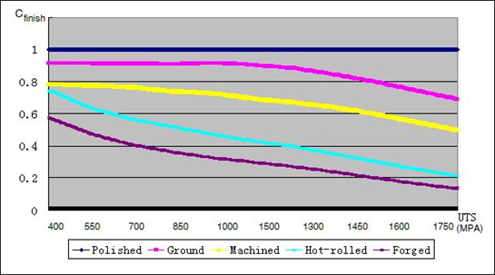
Surface Condition (Finish and Treatment)

Surface condition is an extremely important factor influencing fatigue strength, as fatigue failures nucleate at the surface. Surface finish and treatment factors are considered to correct the fatigue analysis results.

Surface finish correction factor Cfinish is used to characterize the roughness of the surface. It is presented on diagrams that categorize finish by means of qualitative terms such as polished, machined or forged.

fea_surface_finish

Figure 23*: Surface finish correction factor for steels
(* Source: Yung-Li Lee, Jwo. Pan, Richard B. Hathaway and Mark E. Barekey. Fatigue testing and analysis: Theory and practice, Elsevier, 2005)

Surface treatment can improve the fatigue strength of components. NITRIDED, SHOT-PEENED, and COLD-ROLLED are considered for surface treatment correction. It is also possible to input a value to specify the surface treatment factor Ctreat.

In general cases, the total correction factor is Csur = Ctreat * Cfinish.

If treatment type is NITRIDED, then the total correction is Csur = 2.0 * Cfinish (Ctreat = 2.0).

If treatment type is SHOT-PEENED or COLD-ROLLED, then the total correction is Csur = 1.0. It means you will ignore the effect of surface finish.

The fatigue endurance limit FL will be modified by Csur as: FL' = FL * Csur. For two segment S-N curve, the stress at the transition point is also modified by multiplying by Csur.

Surface conditions may be defined on a PFAT Bulk Data entry. Surface conditions are then associated with sections of the model through the FATDEF Bulk Data entry.

Fatigue Strength Reduction Factor

In addition to the factors mentioned above, there are various others factors that could affect the fatigue strength of a structure, e.g., notch effect, size effect, loading type. Fatigue strength reduction factor Kf is introduced to account for the combined effect of all such corrections. The fatigue endurance limit FL will be modified by Kf  as: FL' = FL / Kf

The fatigue strength reduction factor may be defined on a PFAT bulk data entry. It may then be associated with sections of the model through the FATDEF bulk data entry.

If both Csur and Kf  are specified, the fatigue endurance limit FL will be modified as: FL' = FL * Csur / Kf.

Csur and Kf  have similar influences on the E-N formula through its elastic part as on the S-N formula. In the elastic part of the E-N formula, a nominal fatigue endurance limit FL is calculated internally from the reversal limit of endurance Nc. FL will be corrected if Csur and Kf are presented. The elastic part will be modified as well with the updated nominal fatigue limit.
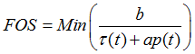
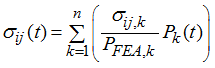
hmtoggle_plus1Setting Up a Fatigue Analysis

Static Fatigue Analysis

Linear Superposition of Multiple FEA/Load Time History Load Cases

When there are several load cases at the same time, all of which vary independently of one another, the principle of linear superposition will be used to combine all load cases together to determine the stress variation at each calculation point due to the combination of all loads. The formula is:

      (73)

Where, n is the total number of load cases, Pk(t) and fea_total_stress_tensor are, respectively, the time variation of the k-th load time history and the total stress tensor, and PFEA,k and fea_stress_tensor are, respectively, the k-th load magnitude and stress tensor from FE analysis.

Transient Fatigue Analysis

During Transient Fatigue Analysis, the load-time history input is not required, as it is calculated internally during Transient Analysis.

Load Time History Compression

This option is used to save calculation time. It will remove small cycles (defined by a gate value) and intermediate points.

fea_small_cycles_removal

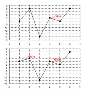
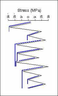
Figure 24: Sample showing removal of small cycles

When removing small cycles, adjacent turning points, where the difference is less than the maximum range multiplied by relative gate value, will be removed from each channel. However, phase relationship will be maintained, when peaks and valleys occur on different channels at different times. This is shown by the sample above. In the first channel (top), the points at time 4 and 5 will be removed when the absolute gate equals one, while in the second channel (bottom), the points at time 1 and 2 will not be removed in order to keep the phase relationship between channels.

fea_intermediate_pts_removal2

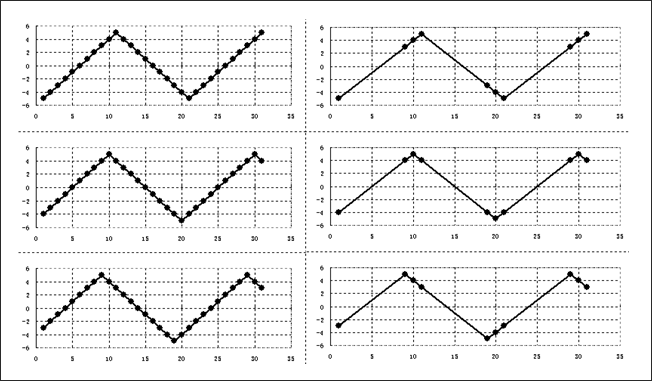
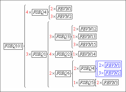
Figure 25: Sample showing removal of intermediate points

Removing intermediate points is another important mechanism to save computation time. If any point on the load-time history is neither a peak nor valley point, it will not contribute in determining any stress cycle. Such points could be screened out in the fatigue computation without losing the accuracy, but the computation time could be saved significantly. For example, the left column in Fig 11 shows three load-time histories of three super-positioned loadcases, respectively. After removing the intermediate points, the three load-time histories are obtained as in the right column, which can produce the same fatigue results as the left column, but use much less time. This mechanism is built in OptiStruct and is effective automatically.

Fatigue Loads, Events and Sequences

Fatigue loading is defined by scaling a static subcase with a load-time history.

A fatigue event consists of one or more static loadcases applied simultaneously in the same time duration scaled by load-time histories. For fatigue events with more than one static loadcase stress, linear superposition is used.

A fatigue sequence consists of a number of fatigue events and repeated instances of these events. A fatigue sequence can be made up of other sub fatigue sequences and/or fatigue events. In this way, you can define very complex events and sequences for fatigue analysis.

In OptiStruct, fatigue sequences defined in fatigue subcases (referred by FATSEQ) are the basic loading blocks. The fatigue life results of these fatigue subcases are calculated as the number of repeats of the loading block.

Below is an example of a "tree-like" fatigue sequence, which can be defined in OptiStruct, with FSEQ# identifying fatigue sequences and FEVN# identifying fatigue events:

fea_tree-like_fatique

Figure 26: Example of a "tree-like" fatigue sequence

Fatigue loading is defined by a FATLOAD Bulk Data entry, where a static subcase and a load-time history are associated.

A fatigue loading event is defined by a FATEVNT Bulk Data entry, where one or more fatigue loads (FATLOAD) are selected.

A fatigue loading sequence is defined by a FATSEQ Bulk Data entry, where a sequence of one or more fatigue loading events or other fatigue loading sequences is given. The appropriate FATSEQ bulk data entry may be referenced from a fatigue subcase definition through the FATSEQ Subcase Information entry.