Fluid-Structure Interaction (Beta)

Introduction

OptiStruct and AcuSolve are fully-integrated to perform a Direct Coupled Fluid-Structure Interaction (DC-FSI) Analysis based on a partitioned staggered approach. OptiStruct and AcuSolve both include time-domain simulation capabilities that break the coupled solution into a number of time steps. Since the governing equations of both OptiStruct and AcuSolve are nonlinear, sub-iterations are typically required within each time step.

fsi_model

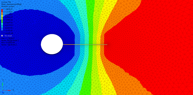
Figure 1: Fluid-Structure Interaction between a solid plate and enclosing fluid.

As the name suggests, Fluid-Structure Interaction simulates the interrelationship between fluid flow and the solid body the fluid is in contact with. The behavior of the structure affects the fluid and vice-versa in a coupled dynamic interaction that is captured by dividing the time domain into time steps. For each time step, the exchanged solution attributes are solved for from the governing equations until equilibrium convergence is attained. Each such iteration run through towards convergence within a time step is known as an exchange (in OptiStruct) or a stagger (in AcuSolve). The fluid flow can be external to the solid object, similar to an aircraft wing moving through air, or it can be internal, like the flow of coolant in a condenser tube.

Target Applications

The Fluid-Structure Interaction capability aims at simulations of dynamic problems subjected to fluid flow interactions and their complex interrelationship. It is recommended to use this direct coupling method when the solid structural response variables affecting the fluid domain vary significantly and result in large changes in the fluid response. In this process, the responses from both domains are exchanged in real time.

Note:

For linear structural response the P-FSI (Practical FSI) solution offered by AcuSolve may be more effective in solving the linearized structural response with the nonlinear flow solution. For further information on the P-FSI method, refer to the AcuSolve Command Reference Manual.

Supported Solutions

A large number of physical state variables affect the interrelationship between the structure and the fluid domains. For example, pressure of the fluid at the interface can affect displacement (and thereby the stress state) of the solid structure, and vice-versa. The displacements at the structural interface can cause changes to fluid flow leading to significant differences in fluid behavior across the entire domain. Similarly, thermal loads on the structure can lead to temperature changes at the structural interface, leading to a changing temperature field for the fluid. Currently, in OptiStruct and AcuSolve the following solutions for the interaction is supported:

•	Structural Fluid-Structure Interaction (Nonlinear Direct Transient Structural Response of the structure).

•	Thermal Fluid-Structure Interaction (Linear Transient Heat Transfer Response of the structure).

Combined structural and thermal heat transfer solutions in conjunction with fluid-structure interaction is currently not supported. You can either run Structural FSI or Thermal FSI, however, you cannot run both in the same run. In the following sections, SFSI refers to Structural Fluid-Structure Interaction and TFSI refers to Thermal Fluid-Structure Interaction for brevity and to avoid redundancy.

Fluid Structure Interaction - Workflow

Fluid-Structure Interaction involves working with two different software's, OptiStruct (the structural solver) and AcuSolve (the fluid solver). You will set up models in both OptiStruct and AcuSolve separately. The following workflow is strongly recommended for running FSI simulations:

1.	Develop the OptiStruct structural model and the AcuSolve-only fluid model, and ensure that the uncoupled analyses run successfully on the corresponding solver.

2.	After each model runs successfully, identify the fluid-structure interface, and include FSI commands to the individual standalone models (see corresponding sections below).

3.	Run the coupled analysis.

4.	Post-process the FSI solution (see Output below).

This workflow ensures that both the OptiStruct and the AcuSolve models are defined properly prior to performing a coupled simulation. OptiStruct and AcuSolve do not require that the analysis be run with a particular unit system, but both analyses require you to use a consistent unit system. As a rule, all quantities exchanged between the two solvers will be in dimensional form, and the components of all vector quantities will be resolved in the inertial frame. For consistency, identical inertial frames must be selected for OptiStruct and AcuSolve.

OptiStruct Model

Preparing the OptiStruct model for FSI involves the following recommendations:

1.	Create an OptiStruct input file.

Identify the interface region and the solution variables exchanged between OptiStruct and AcuSolve (this depends on the type of coupled solution you are running, for example, SFSI or TFSI. For SFSI, the nodal displacements are provided as input to AcuSolve, which in turn provides pressure as input to OptiStruct).

Define the port number to be used by OptiStruct and AcuSolve for communication. The OptiStruct input data is described by the FSI Bulk Data Entry (which is referenced in the subcase section by the FSI Subcase Information Entry). Each of the data fields are discussed below in their relevant sections.

AcuSolve Model

This section provides an overview for preparing the AcuSolve model for FSI. For detailed information on the commands, refer to the AcuSolve Command Reference Manual. The recommendations to prepare the AcuSolve model are:

1.	Create an AcuSolve input file.

2.	Set the analysis parameters to include an external field.

3.	Define the solution strategy.

4.	Define the external surface definition.

Setting Analysis Parameters to Include an External Field

In the AcuSolve model, use the EQUATION command to specify the solution fields available or the system of equation that are present in the problem. To include a field that is computed with an external solver, for OptiStruct, set the external_code parameter to 'ON'.

EQUATION {

flow	= <flow type>

mesh	= <mesh type>

external_code

= on

}

The mesh parameter determines the type of mesh at the interface. This depends on the type of information exchanged at the interface and the boundary conditions. For Thermal FSI, currently, only heat transfer is supported, and therefore, this parameter should be set to Eulerian since the mesh is fixed. For Structural FSI, there is an exchange of displacements and pressure at the interface and in addition, mesh displacement and velocity boundary conditions are present. Therefore, the mesh parameter should be set to Arbitrary Lagrangian Eulerian. See the corresponding FSI User’s Guide pages for more information regarding boundary conditions at the interface.

Fluid-Structure Interface

Structure:

The structural interface of the solid model that is in contact with the fluid domain is known as a damp surface. The damp surface of the structural mesh must be selected in the OptiStruct input data (FSI Bulk Data Entry). The damp surface can either be specified by a surface (SURFID field) or a group of elements (ELSET field). Note that the structural mesh on the damp surface does not have to match the interfacing fluid mesh. AcuSolve will internally project the flow variables (pressure for SFSI, heat flux for TFSI) from the fluid interface mesh onto a non-matching damp surface structural mesh to formulate loading. The mapping of nodal data (pressure or flux) is also supported for structural beam elements. For example, a rod, pipe or blade can be modeled with simple beam elements in the structural mesh. The corresponding fluid mesh will contain the actual three-dimensional geometry of these beam elements.

The damp surface can be specified by a group of elements (ELSET field) or the OptiStruct SURF entry (referenced on the SURFID field). The SURF entry has many options that can be used to specify a surface. The surface can be either the surface of a shell structure or the surface of a solid mesh. Note that beam elements cannot be specified using the SURF data. If the damp surface consists of beam elements, then these must be specified as a beam element set.

The matching fluid interface is specified in the AcuSolve data using the EXTERNAL_CODE_SURFACE command. For further information on AcuSolve data, refer to the AcuSolve Command Reference Manual.

Fluid:

Use the EXTERNAL_CODE_SURFACE command to define the interface between the fluid interface and corresponding parameters. The command specifies the surface topology, as well as the interface proprieties.

Depending on the problem being solved (SFSI or TFSI), various parameters are available to define the interface behavior. A few of them that are relevant to the corresponding solution type are discussed in the respective SFSI and TFSI User’s Guide pages. For detailed information on the different parameters, refer to the AcuSolve Command Reference Manual.

Scaling of Quantities

You may apply a multiplier function in AcuSolve to the solution variables (displacement/temperature) from OptiStruct. Scaling fields may be useful when starting a fluid-structure interaction simulation with high inertial effects. Specify a multiplier function on the EXTERNAL_CODE command. An example ramping multiplier function and its usage is shown below:

MULTIPLIER_FUNCTION("ramp" ) {

type	= <piecewise_linear>

curve_fit_values

= { 1, 0.0 ; 10 , 1 }

curve_fit_variable

= time_step

}

EXTERNAL_CODE {

…

multiplier_function

= "ramp"

…

}

Communication between OptiStruct and AcuSolve

OptiStruct and AcuSolve can be run on heterogeneous and remote platforms which are located on the same network domain. The communication between OptiStruct and AcuSolve is via sockets. To start a coupled simulation between OptiStruct and AcuSolve, one of them should be run first to initiate the communication process, while the other will subsequently connect to the initiated communication process.

Communication Initiation

In OptiStruct the socket port number is specified by the PORT field of the FSI Bulk Data Entry. The default port number is 10000. This same port number must be specified in the socket_port entry of the EXTERNAL_CODE block in the AcuSolve input file (filename.inp). If the machine that OptiStruct is running on is named machine1, then the EXTERNAL_CODE will look like:

EXTERNAL_CODE {

communication

= socket

socket_initiate

= no

socket_host

= "machine1"

socket_port

= 10000

}

OptiStruct and AcuSolve should be started independently. OptiStruct will wait for AcuSolve to initiate the socket connection (or vice-versa). The time that OptiStruct will wait (in seconds, after pre-processing is complete) is determined by the WAITTIME field on the FSI Bulk Data Entry (the default value is 3600 seconds). Similarly, the time (in seconds, after pre-processing is complete) that AcuSolve will wait until OptiStruct initiates communication at the socket is determined by the external_code_wait_time field in the Acusim.cnf file (or the –ecwait run option).

The wait time counting is initiated after pre-processing of the input file in both OptiStruct and AcuSolve. The following example schematic illustrates one scenario wherein OptiStruct is initiated first and waits for AcuSolve.

fsi_optistruct_starts_first

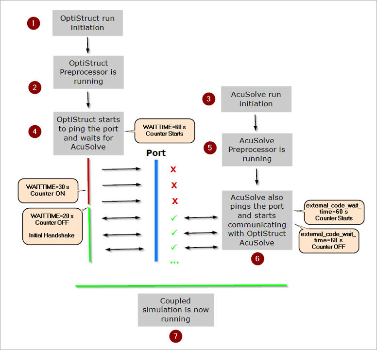
Figure 2: Example schematic showing FSI initiation when OptiStruct starts first

The wait time input by you determines the time the solver will wait until the initial handshake. After this initial handshake, the wait time no longer applies. When the wait time specified expires, and the second solver has still not begun communication with the first, then the solver that was started first will error out. An example schematic is shown below:

fsi_acusolve_not_started

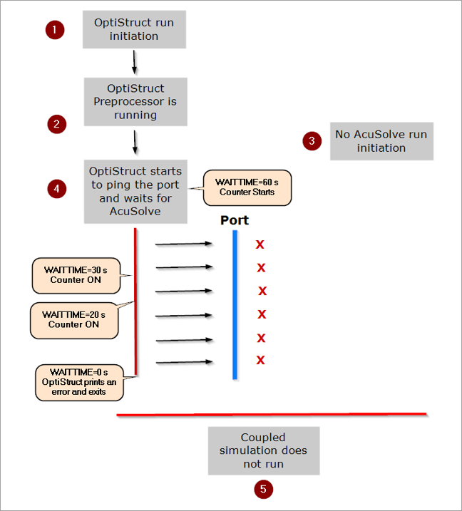
Figure 3: No initial handshake. AcuSolve is not started, so OptiStruct exits the solution after the wait time expires.

Before the start of the time step loops, basic information about the interface must be exchanged between the two software. First, a number of parameters controlling the interface strategy must be set for both. Second, the physical parameters of the interface must be defined.

Time Steps and Data Exchanges

For AcuSolve, in conjunction to the EQUATION command, which specifies the existence of solution fields in the problem, you must use TIME_SEQUENCE and STAGGER commands to define time stepping and staggering strategy. The preferred method is to use the AUTO_SOLUTION_STRATEGY command to have AcuSolve generate the solution strategy commands. For OptiStruct, the data exchange parameters are available on the FSI Bulk Data Entry and time stepping data is specified on the NLPARM, TSTEP, or TSTEPNL entries (depending upon the type of solution or data). See the corresponding SFSI or TFSI User’s Guide pages for more information.

Both OptiStruct and AcuSolve need to use the same time step size and the total number of time steps should be the same. Also, the size of the time step needs to remain constant in both OptiStruct and AcuSolve. For example, for 100 time steps of 0.001 seconds each the OptiStruct and AcuSolve data are:

AUTO_SOLUTION_STRATEGY {

initial_time_increment

= 0.001

max_time_steps

= 101

min_stagger_iterations

= 1

max_stagger_iterations

= 20

}

and

(1)	(2)	(3)	(4)	(5)	(6)	(7)	(8)	(9)	(10)
NLPARM	5	40	1.0e-3			80	UP
	1.0e-2	1.0e-5
		1.0e-1

Note:

For AcuSolve the maximum number of time steps set should be one greater than the maximum number of times steps set for the corresponding OptiStruct model.

At each time step, solution variables (displacement/pressures for SFSI, temperature/flux for TFSI) are exchanged between OptiStruct and AcuSolve until they converge to a certain tolerance. Once convergence is achieved, the analysis continues on to the next time step. These exchanges are called "staggers" in AcuSolve. The minimum number of staggers (called exchanges in OptiStruct) can be specified by the min_stagger_iterations parameter in the AcuSolve AUTO_SOLUTION_STRATEGY block, this is also influenced by other AcuSolve run parameters. The minimum number of exchanges in OptiStruct can be specified by the MINEX field in the OptiStruct FSI Bulk Data Entry.

The maximum number of staggers is set by the max_stagger_iterations parameter in the AcuSolve AUTO_SOLUTION_STRATEGY block, this is also influenced by other AcuSolve run parameters. The maximum number of exchanges in OptiStruct can be specified by the MAXEX field in the FSI Bulk Data Entry.

The maximum or minimum number of exchanges (MAXEX/MINEX) is set in the OptiStruct model. There may be multiple locations within the AcuSolve model, where the maximum/minimum number of staggers are defined. The FSI run will use the lowest maximum number of exchanges/staggers and the highest minimum number of exchanges/staggers out of all available such specified data. Therefore, depending on AcuSolve, each time increment may end within a subset space lesser than or equal to [MINEX,MAXEX].

The solution variable convergence tolerances are used to reduce the number of exchanges/staggers to that required receive stable and accurate results. This may significantly reduce run times while generating results. The solution variable tolerances are specified by the FCNVTOL, DCNVTOL, TCNVTOL, and FXCNVTOL fields on the FSI Bulk Data Entry. If these tolerances are set high, the solution time will be reduced, but solution accuracy may also be affected. The convergence_tolerance parameter can also be used to define convergence tolerances in the AcuSolve input data.

Input

In this section the general input for any FSI run is discussed. For detailed information regarding specific SFSI/TFSI input data, refer to the corresponding document. In OptiStruct-AcuSolve FSI, you typically only need to define the fluid-structure interface to run Fluid-Structure Interaction Analysis.

For example, in OptiStruct, if the interface surface has a SURF ID of 10, the input data would be:

FSI,2,10

In this case, all of the other parameters are set to their default values.

In order to reduce run times, it is recommended to set an upper bound on the number of exchanges/staggers, as well as setting higher values for the solution variable convergence tolerances.

For example, in OptiStruct, set the maximum number of exchanges to 5 and the force and displacement convergence tolerances to 0.01 respectively with the data:

FSI,2,10,,,,0.01,0.01

The FSI Bulk Data Entry in OptiStruct should be referenced in the Subcase Information section by a corresponding FSI Subcase Information Entry. Currently, only one FSI Subcase Entry can be specified in a model (in other words, within a model containing multiple subcases, only one subcase can have the FSI subcase entry). See Limitations for further information.

Model Location:

The OptiStruct and AcuSolve models must be co-located. In other words, fluid boundary mesh and the corresponding structural damp surface mesh match each other as a physical boundary. The gap between these meshes should be small. To verify the conformity of exchange surfaces in AcuSolve, consult the .log file for the structural mesh information, as shown below. Verify the number of damp surface elements and the minimum and maximum coordinates of the damp surface, as well as for matching bounding box and areas to help identify position, size and orientation mismatch:

acuSolve: No. external code nodes = 170

acuSolve: No. external code tri3s = 0

acuSolve: No. external code quad4s = 168

acuSolve: No. external code tri6s = 0

acuSolve: No. external code line2s = 0

acuSolve: Min/Max x-coord = -2.500000e-001 2.500000e-001

acuSolve: Min/Max y-coord = 0.000000e+000 2.000000e+000

acuSolve: Min/Max z-coord = -2.500000e-001 2.500000e-001

acuSolve: Total surface area = 4.500000e+000

acuSolve: Total length = 0.000000e+000

acuSolve: No. external code mbds = 0

acuSolve: No. fluid wet surfaces = 18

acuSolve: Min/Max x-coord = -2.500000e-001 2.500000e-001

acuSolve: Min/Max y-coord = 0.000000e+000 2.000000e+000

acuSolve: Min/Max z-coord = -2.500000e-001 2.500000e-001

acuSolve: Total fluid surface area = 2.250000e+000

Running FSI

The OptiStruct and AcuSolve runs can be run either in serial or parallel mode. As explained in the previous sections, you simply initiate an OptiStruct or AcuSolve run and then start the second subsequent run. OptiStruct and AcuSolve will communicate via the specified port and exchange the required information with each other.

OptiStruct and AcuSolve may be run in parallel on distributed memory clusters. Both MPI and OpenMP parallelization modes are currently supported. For more information, refer to High Performance Computing.

General Limitations

1.	If the structural interface surface contains beam elements, no other elements can be used to define the damp surface. In other words, beam elements cannot be mixed with other elements to define the damp surface.

2.	Quadratic and modified tetrahedral elements are currently not supported.

3.	A constant fixed time step should exist between the two solvers.

Activity Timeline

OptiStruct

AcuSolve

FSI Initiation

Set up standalone OptiStruct model co-located with the fluid domain

Set up standalone AcuSolve model
co-located with the structural domain

Standalone verification

Run independently on OptiStruct to verify model integrity

Run independently on AcuSolve
to verify model integrity

Identifying the interface

Identify the structural damp interface that is in contact with the fluid domain as a SURF entry or an element SET

Identify the fluid interface that is in contact with the structural domain as an element set

Referencing the interface

Set up FSI Bulk Data Entry and reference the interface on the SURFID or ELSET fields

Set up EXTERNAL_CODE_SURFACE

Command block and reference the interface elements using the element_set parameter

Modeling interface behavior

The USETAG field on the FSI Bulk Data Entry can be used to tag damp surfaces

The EXTERNAL_CODE_SURFACE

Command block can be used to define parameters to model interface behavior like velocity_type, mesh_displacement_type, temperature_type,
and so on.
For additional information, refer to the corresponding solution page (SFSI/TFSI).

Activating FSI

The FSI Subcase Information Entry can be used to reference the FSI Bulk Data Entry

The external_code parameter is set to on in the EQUATION command block to activate the use of an external solver (OptiStruct) to provide the solution field.

Identifying communication protocols

The PORT and WAITTIME fields on the FSI Bulk Data Entry are used to identify the socket and the time OptiStruct waits for AcuSolve.

The EXTERNAL_CODE command block is used to identify the socket and machine for communication.
The external_code_wait_time

parameter can be defined in the Acusim.cnf file to define the time AcuSolve waits for OptiStruct.

Specify run control parameters

The FCNVTOL, DCNVTOL, TCNVTOL, and FXCNVTOL fields on the FSI Bulk Data Entry can be used to adjust exchange convergence tolerances.

The MINEX and MAXEX fields control the minimum and maximum number of exchanges per time step

The INITTS field identifies the initial AcuSolve time increment to start the coupling with OptiStruct

The convergence_tolerance parameter in the AUTO_SOLUTION_STRATEGY command block can be used to determine the stagger convergence tolerances.

The min_stagger_iterations and max_stagger_iterations parameters in the same command block define the minimum and maximum staggers per time step.

There are additional sections of the AcuSolve run where the minimum and maximum number of exchanges are defined.

Running FSI

Run the OptiStruct input file (with FSI data) and look for the cci.txt file in the working directory

After starting the OptiStruct run, initiate the AcuSolve run before the specified wait time. If the runs are proceeding as expected, you should see exchange/stagger information printed to:

1. The OptiStruct .out file

2. The AcuSolve .log file

3 The cci.txt file – a log of the exchange/stagger data is printed

Note:

1.	Either OptiStruct or AcuSolve can be started first. The critical step is to initiate the second solver prior to the expiration of the wait time (for initial handshake) after the first one is started.

If the wait time is set to a reasonable value (say, 10 minutes), and both models do not progress beyond the pre-processing stage and the cci.txt file does not contain printed information, then check to make sure that the socket_host and socket_port are set correctly in the AcuSolve model and that socket_port matches the PORT field on the FSI Bulk Data Entry in the OptiStruct model.

FSI output

An .h3d file is generated with the structural results at the end of the simulation

The AcuSolve .log file is available to post-process the results of the simulation and can be loaded into HyperView.

Note: Currently, the structural and fluid TFSI results can be overlaid; however, the SFSI results can only be post-processed separately.

Table 2: Fluid-Structure Interaction Complete Setup Timeline

Output

The FSI results are output to the corresponding working directories. The structural (OptiStruct) results are output to the H3D file by default and can be post-processed in HyperView. However, this file will not contain the fluid results. The fluid results are available in the AcuSolve .log file in the AcuSolve working directory. The AcuSolve .log file can also be loaded into HyperView. A cci.txt file is output by default for an FSI run, which contains information pertaining to model progression. Logs regarding connection establishment, initial external code handshake and subsequent time step data in conjunction with exchange/stagger information are printed to the cci file.

See the corresponding FSI solution page for more information about post-processing.