Contacts Post-Processing

This section summarizes the post-processing capabilities that are available in MotionView, HyperView, and HyperGraph for contact models. MotionSolve generates two files; the H3D and the ABF as output. The H3D output file is used by HyperView to visualize results. The ABF (or alternatively, PLT or MRF) file is used for plotting responses in HyperGraph. MotionView provides an automatic way of generating animation and plot pages for some common type of results after a contact simulation.

HyperView – Contact Overview

The contact overview capability is particularly useful, if you want to see where contact occurred during the entire simulation and what the maximum penetration depths were. These help you to understand how the contacts are behaving.

The Contact Overview capability in HyperView allows you to visualize in one frame a contour of the maximum penetration depth during the entire simulation for each element in contact.

Reviewing Maximum penetration depth

The steps to access the contact overview results for the simulation are:

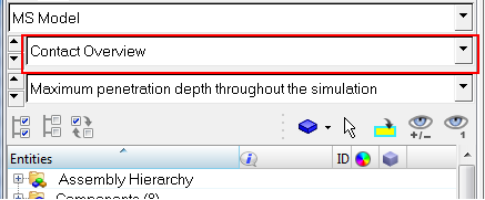
1.	Select Contact Overview in the Results browser in the left of the window:

contacts_post_proc_hv_res_brwsr_mv

2.	Select the Contour button in the toolbar:

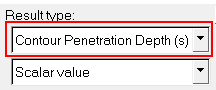
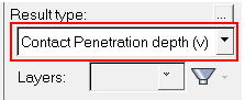
3.	Select the Contour Penetration Depth (s) for the Result type in the panel:

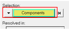
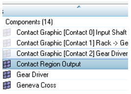
contacts_post_proc_hv_contour_panel_res_type_mv

4.	Select Components in the Selection input collector:

contacts_post_proc_hv_contour_panel_cmpnt_input_slctr_mv

5.	Select the graphics in the graphics window.

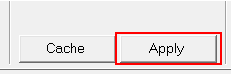
contacts_post_proc_hv_model_example_mv

6.	Click Apply.

contacts_post_proc_hv_contour_panel_apply_button_mv

7.	Inspect the results.

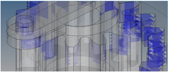
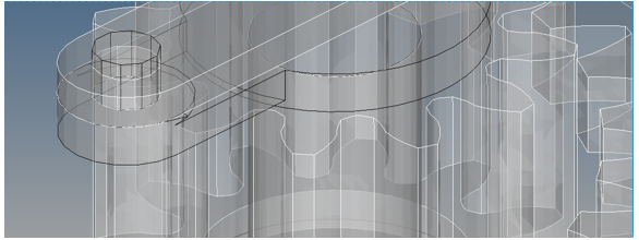
contacts_post_proc_hv_model_example2_mv

Tip

The overview results are best seen if you change the opacity of the body graphics:

-	Select the opacity tool in the toolbar and select Transparent Elements and Feature Lines from the drop-down menu.

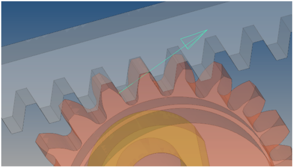
contacts_post_proc_hv_trans_elem_ftre_lines_icon_mv

HyperView – Visualizing Transient Results

Vector results are displayed as arrows. The length of the arrow denotes the magnitude of the vector and the direction of the arrow is along the direction of the vector result. Colors are used to provide a further visual cue. Large vectors are colored red and small vectors blue. Intermediate rainbow colors are used to color intermediate sized results.

Available results

The following different types of vector results are available for visualization for each point in time:

Contact Normal Force	The normal force on each triangle.
Contact Penetration Depth	The penetration depth vector on each triangle.
Contact Penetration Velocity	The penetration velocity vector on each triangle.
Contact Point Slip Velocity	The slip velocity vector at the contact point on each triangle.
Contact Tangential Force	The frictional force on each triangle.
Contact Total Force	The total force on each triangle (normal + tangential).

Accessing Vector Results

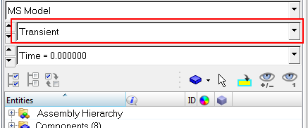
1.	Select Transient in the Results browser.

contacts_post_proc_hv_res_brwsr_transient_mv

2.	Select the Vector button in the toolbar.

3.	Begin the animation of the results by clicking the play button.

4.	Select the Result type of interest. Animation penetration depth, contact forces, and velocities are all described as examples in the sections below.

Reviewing Penetration Depth

1.	Follow the previous steps (listed above in the Accessing Vector Results section) to access the vector results.

2.	Select Contour Penetration Depth (v) for the Result type in the panel.

contacts_post_proc_hv_vector_panel_res_type_mv

3.	Click the Apply button.

contacts_post_proc_hv_vector_panel_apply_button_mv

4.	Inspect the results in the graphics area.

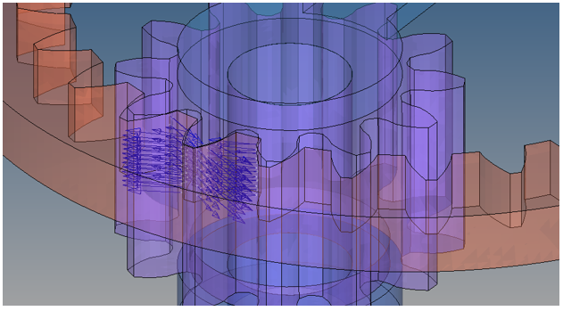
contacts_post_proc_hv_model_example3_mv

Reviewing Contact Forces

1.	Follow the previous steps (listed above in the Accessing Vector Results section) to access the vector results.

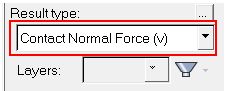
2.	Select the Contact Normal Force (v) for the Result type in the panel:

contacts_post_proc_hv_vector_panel_res_type_nrml_frce_mv

Other contact force options include:

•	Contact Tangential Force (v) – the vector sum of the normal and tangential forces.

3.	Click the Apply button.

contacts_post_proc_hv_vector_panel_apply_button_mv

4.	Inspect the results in the graphics area.

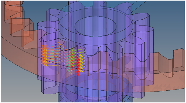
contacts_post_proc_hv_model_example4_mv

By default the contact force results are displayed at each element (of the first body in the contact pair) in contact.

5.	To visualize force as a sum at a particular region of contact, turn on the component Contact Reqion Output, by clicking on it in the browser. Next, turn off all other components with labels starting with Contact Graphics.

contacts_post_proc_hv_res_brwsr_contact_graphics_mv

6.	Use the above mentioned steps to apply a display of the forces in the graphics area.

contacts_post_proc_hv_model_contact_graphics_example_mv

Reviewing Contact Velocities

1.	Follow the previous steps (listed above in the Accessing Vector Results section) to access the vector results.

2.	Select Contact Point Slip velocity (v) for the Result type in the panel.

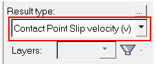
contacts_post_proc_hv_vector_panel_res_type_slip_vel_mv

The other contact velocity option is Contact Penetration Velocity (v)

3.	Click the Apply button.

contacts_post_proc_hv_vector_panel_apply_button_mv

4.	Inspect the results in the graphics area.

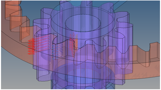
contacts_post_proc_hv_model_example5_mv

Tip

The vector results are best seen if you change the opacity of the body graphics:

-	Select the opacity tool in the toolbar and select Transparent Elements and Feature Lines.

contacts_post_proc_hv_trans_elem_ftre_lines_icon_mv

HyperGraph – Plotting Contact Results

For each contact you define in MotionView, two contact REQUESTS are automatically written to the XML file for MotionSolve. As a part of its post-simulation activities, MotionSolve will write out the data associated with these REQUESTS to the output file(s) you selected.

Contact results are written to the ABF, MRF, and PLT files. The same contact information is available in each file.

•	The first REQUEST contains the net force and torque experienced by the reference MARKER associated with the I-Geometry of the contact.

•	The second REQUEST contains the net force and torque experienced by the reference MARKER associated with the J-Geometry of the contact.

For each REQUEST the following time histories are available:

F1	The magnitude of the total contact force experienced by the reference MARKER.
F2	The X-component of the total contact force experienced by the reference MARKER, as computed in the coordinate system of the RM MARKER of the REQUEST. When not specified, the RM MARKER defaults to the global coordinate system.
F3	The Y-component of the total contact force experienced by the reference MARKER, as computed in the coordinate system of the RM MARKER of the REQUEST. When not specified, the RM MARKER defaults to the global coordinate system.
F4	The Z-component of the total contact force experienced by the reference MARKER, as computed in the coordinate system of the RM MARKER of the REQUEST. When not specified, the RM MARKER defaults to the global coordinate system.
F5	The magnitude of the total contact torque experienced by the reference MARKER. The non-zero moment arm of the vector from the REFERENCE MARKER to each contact point causes this torque.
F6	The X-component of the total contact torque experienced by the reference MARKER, as computed in the coordinate system of the RM MARKER of the REQUEST. When not specified, the RM MARKER defaults to the global coordinate system.
F7	The Y-component of the total contact torque experienced by the reference MARKER, as computed in the coordinate system of the RM MARKER of the REQUEST. When not specified, the RM MARKER defaults to the global coordinate system.
F8	The Z-component of the total contact torque experienced by the reference MARKER, as computed in the coordinate system of the RM MARKER of the REQUEST. When not specified, the RM MARKER defaults to the global coordinate system.

Plotting Contact Forces

The steps to plot the contact force results for the simulation are:

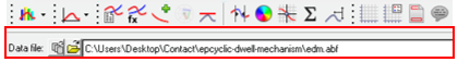
1.	Load the desired results file into HyperGraph:

contacts_post_proc_hg_load_file_mv

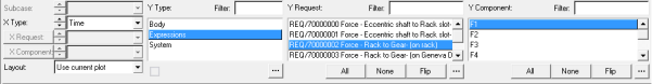
2.	Select the Y Type as Expression, the relevant Y Request, and the Y Component belonging to the contact force:

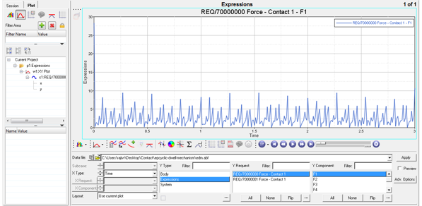
contacts_post_proc_hg_plots_panel_mv

3.	Click the Apply button.

4.	Inspect the results in the graphics area.

contacts_post_proc_hg_plot_example_mv

MotionView – View Reports

MotionView comes with a standard report for contact simulation that adds commonly visualized results to the HyperWorks session.

Generating an automated contact report

Once the simulation submitted via the MotionView Run panel is completed, follow the steps below:

1.	From the Analysis menu, click View Reports.

mv-1012_analysis_menu_view_reports

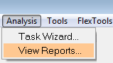
The View Reports dialog is displayed.

contacts_post_proc_view_reports_mv

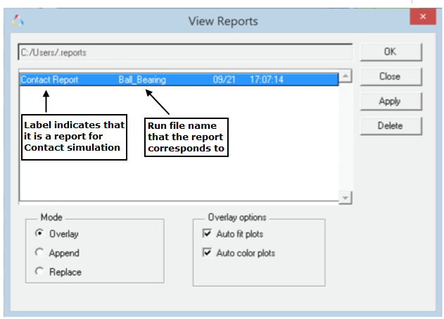
The report item (Contact Report for the last submitted run) will be listed at the top.

2.	Select the item and click OK.

The following pages with results, described in earlier sections, are added to the report. Use the Previous Page/Next Page icons buttons (located at the upper right corner of the window, below the menu bar area and above the graphics area), to view these pages:

•	Contact Force Animation - Contact Region Output

•	Contact Overview

•	Penetration Depth Animation

•	Contact Force Plots