Diagnostics assist in assessing the accuracy of a Fit.
In the Diagnostic tab, quantities are displayed in three columns.
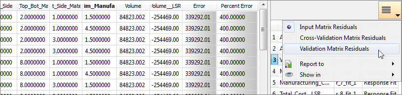
| 1. | The Input Matrix column shows the diagnostic information using only the input matrix. For methods which go through the data points, such as HyperKriging or Radial Basis Functions, input matrix diagnostics are not useful. |
| 2. | The Validation Matrix column compares the approximate model, which was built using the input matrix, against a separate set of user supplied points. Using a validation matrix is the best method to get accurate diagnostic information. |
| 3. | The Cross-Validation Matrix column shows the diagnostic information using a k-fold scheme, which means input data is broken into k groups. For each group, the group's data is used as a validation set for a new approximate model using only the other k-1 group's data. This allows for diagnostic information without the need of a validation matrix. |
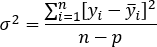
The following definitions are useful in describing diagnostic concepts. For a given set of  input values, denoted as input values, denoted as  , the Fit predictions at the same points are denoted as , the Fit predictions at the same points are denoted as  . The mean of the input values is expressed . The mean of the input values is expressed  . For a Least Squares Regression, p is the number of unknown coefficients in the regression. . For a Least Squares Regression, p is the number of unknown coefficients in the regression.
The following three values are defined as follows:
Total sum of Squares
|
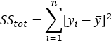
|
Explained Sum of Square
|
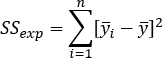
|
Residual Sum of Squares
|
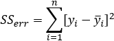
|
Average Absolute Error
|
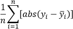
|
Standard deviation
|
|
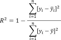
R-Square
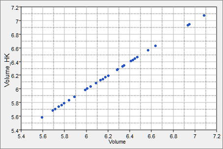
R-Square, commonly called the coefficient of determination, is a measure of how well the Fit can reproduce known data points. Graphically, this can be visualized by scatter plotting the known values versus the predicted values. If the model perfectly predicts the known values, R-Square will have its maximum possible value of 1.0, and the scatter points will lie on a perfect diagonal line, as shown in the image below.
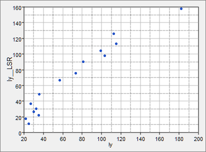
More typically, the Fit introduces modeling error, and the scatter points will deviate from the straight diagonal line, as shown in the image below.
The value of R-Square decreases as errors increase and the scatter plot deviates more from a straight line. The main interpretation of R-Square is that it represents the proportion of variance within the data which is explained by the Fit. For example, if R-Square = 0.84, then 84% of the variance in the data is predictable by the Fit. The higher the value of R-Square, the better the quality of the Fit. In practice, a value above 0.92 is often very good and a value lower than 0.7 necessitates investigation using other metrics. If R-Square is 1.0, you should be skeptical of this result unless the data was expected to be perfectly predicted by the Fit. There are some cases in which R-Square can be negative. A negative R-Square value indicates that using the raw mean would be a better predictor than the Fit itself; the Fit is very poor quality.
In the work area, these numbers are presented with a spark line to indicate the relative value of the number (values typically vary between 0 and 1). Values are color coded based on the following:
| • | When R2 is less than 0.65 (R2 < 0.65) it is displayed red, which indicates the value is not good. |
| • | When R2 is between 0.8 and 0.995 (0.8 < R2 < 0.995) it is displayed green, which indicates the value is good. |
| • | Otherwise it is displayed black, which indicates that you should apply judgment when determining whether the value is or is not good. |
R-Square is defined as:
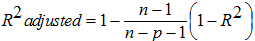
R-Square Adjusted (Least Squares Only)
Due to its formulation, adding a variable to the model will always increase R-Square. R-Square Adjusted is a modification of R-Square that adjusts for the explanatory terms in the model. Unlike R-Square, R-Square Adjusted increases only if the new term improves the model more than would be expected by chance. The adjusted R-Square can be negative, and will always be less than or equal to R-Square. If R-Square and R-Square Adjusted differ dramatically, it indicates that non-significant terms may have been included in the model.
R-Sqaure Adjusted is defined as:
In the work area, these numbers are presented with a spark line to indicate the relative value of the number (values typically vary between 0 and 1). Values are color coded based on the following:
| • | When R2 adjusted is less than 0.65 (R2 adjusted < 0.65) it is displayed red, which indicates the value is not good. |
| • | When R2 adjusted is between 0.8 and 0.995 (0.8 < R2 adjusted < 0.995) it is displayed green, which indicates the value is good. |
| • | Otherwise it is displayed black, which indicates that you should apply judgment when determining whether the value is or is not good. |
Multiple R (Least Squares Only)
Multiple R is the multiple correlation coefficient between actual and predicted values, and in most cases it is the square root of R-Square. It is an indication of the relationship between two variables.
Regression Equation (Least Squares Only)
The complete formula for the predictive model as a function of the input variables.
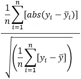
Relative Average Absolute Error
A comparison of the average predicted error and the spread in the data itself. A low ratio is more desirable as it indicates that variance in the Fit’s predicted values are dominated by the actual variance in the data and not by error.
Relative Average Absolute Error is defined as:
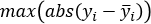
Maximum Absolute Error
The maximum difference, in absolute value, between the observed and predicted values. For the input and validation matrices, this value can also be observed in the Residuals tab.
Maximum Absolute Error is defined as:
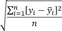
Root Mean Square Error
A measure of weighted average error. A higher quality Fit will have a lower value.
Root Mean Square Error is defined as:
Number of Samples
The number of data points used in the diagnostic computations.
Confidence Intervals (Least Squares Only)
Confidence intervals consist of an upper and lower bound on the coefficients of the regression equation. Bounds represent the confidence that the true value of the coefficient lies within the bounds, based on the given sample.
Enter a specific confidence value in the field that displays when you click  , as shown in the image below. , as shown in the image below.

A higher confidence value will result in wider bounds; a 95% confidence interval is typically used. T-value is defined as:

where βj is the corresponding regression coefficient (the Values column) and SE is the standard error. The standard error is defined as:
SE = 
and:
where Cjj is the diagonal coefficient of the information matrix used during the regression calculation.
P-values are computed using the standard error and t-value to perform a student’s t-test. The p-value indicates the statistical probability that the quantity in the Value column could have resulted from a random sample and that the real value of the coefficient is actually zero (the null hypothesis). A low value, typically less than 0.05, leads to a rejection of the null-hypothesis, meaning the term is statistically significant.
|