|
»Click here to display Table of Contents«
|

CTRIA6 |

|

|

|

|
|
CTRIA6 |
|
|

|

|
|
»Click here to display Table of Contents«
|
CTRIA6 |
|
|
|
|
|
CTRIA6 |
|
|
|
|
Bulk Data Entry
CTRIA6 – Curved Triangular Shell Element Connection
Description
Defines a curved triangular shell element with six grid points.
Format
(1) |
(2) |
(3) |
(4) |
(5) |
(6) |
(7) |
(8) |
(9) |
(10) |
CTRIA6 |
EID |
PID |
G1 |
G2 |
G3 |
G4 |
G5 |
G6 |
|
|
THETA |
ZOFFS |
T1 |
T2 |
T3 |
|
|
|
|
|
Field |
Contents |
EID |
Unique element identification number. No default (Integer > 0) |
PID |
Identification number of a PSHELL, PCOMP or PCOMPP entry. Default = EID (Integer > 0) |
G1,G2,G3 |
Grid point identification numbers of connected corner points. No default (Integers > 0, all unique) |
G4,G5,G6 |
Grid point identification number of connected edge points. Cannot be omitted. No default (Integer > 0 or blank) |
THETA |
Material orientation angle in degrees. Default = 0.0 (Real) |
MCID |
Material coordinate system identification number. The x-axis of this material coordinate system is determined by projecting the x-axis of the MCID coordinate system (defined by the CORDij entry or zero for the basic coordinate system) onto the surface of the element. Default is THETA = 0.0 (Integer > 0) |
ZOFFS |
Offset from the surface of grid points to the element reference plane (Comment 6). Overrides the ZOFFS specified on the PSHELL entry. Default = 0.0 (Real, Character Input = TOP/BOTTOM, or blank) |
Ti |
Membrane thickness of element at grid points G1 through G3. The thickness of the element with Ti specified will be constant and equal to an average of T1, T2, and T3. For defaults: see comment 4. (Real > 0.0 or blank) |
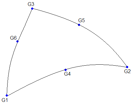
| 1. | Grid points G1 through G6 must be numbered as shown here: |
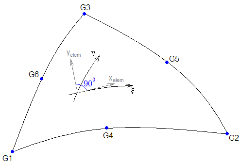
| 2. | The element coordinate system is a Cartesian system defined locally for each point ( |
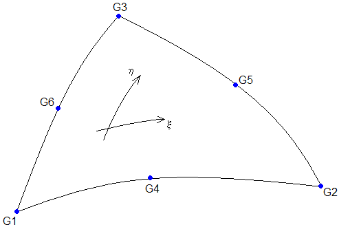
It is based on the following rules:
| - | The plane containing xelem and yelem is tangent to the surface of the element. |
| - | xelem is tangent to the line of constant |
| - | xelem increases in the general direction of increasing |
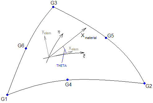
| 3. | The orientation of the material coordinate system is defined locally at each interior integration point by THETA, which is the angle from the line of constant |
If MCID is used in place of THETA, then the local material x-direction (Xmaterial) is obtained at any point in the element by projection of the x-axis of the MCID coordinate system onto the surface of the element at this point. The local z-direction is aligned with the normal to the surface and the material y-direction (Ymaterial) is constructed accordingly to produce right-handed local material system X-Y-Zmaterial.
| 4. | T1, T2, and T3 are optional. If they are not supplied, the element thickness will be set equal to the value of T on the PSHELL entry. If 0.0 is specified for Ti, the thickness at that node is zero. If Ti is supplied, PID cannot reference PCOMP or PCOMPP data. If the property referenced by PID is selected as a region for Size optimization, then any Ti values defined here are ignored. If you input Ti for elements in the design space for Topology or Free-Size optimization, the run will error out. |
| 5. | It is required that the midside grid points be located within the middle third of the edge. That is the interval (0.25, 0.75) excluding the quarter points 0.25 and 0.75. If the edge point is located at the quarter point, the program may fail with an error or the calculated stresses will be meaningless. |
| 6. | The shell reference plane can be offset from the plane defined by element nodes by means of ZOFFS. In this case all other information, such as material matrices or fiber locations for the calculation of stresses, is given relative to the offset reference plane. Similarly, shell results, such as shell element forces, are output on the offset reference plane. |
ZOFFS can be input in two different formats:
| 1. | Real: |
A positive or a negative value of ZOFFS is specified in this format. A positive value of ZOFFS implies that the reference plane of each shell element is offset a distance of ZOFFS along the positive z-axis of its element coordinate system.
| 2. | Surface: |
This format allows you to select either “Top” or “Bottom” option to specify the offset value.
Top:
The top surface of the shell element and the plane defined by the element nodes are coincident.
This makes the effective "Real" ZOFFS value equal to half of the thickness of the PSHELL property entry referenced by this element. (The sign of the ZOFFS value would depend on the direction of the offset relative to the positive z-axis of the element coordinate system, as defined in the Real section). See Figure 1.
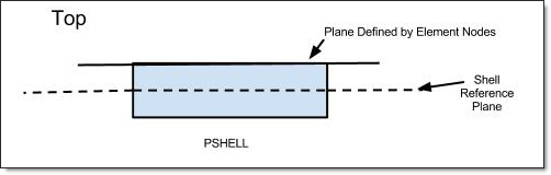
Figure 1: Top option in ZOFFS
Bottom:
The bottom surface of the shell element and the plane defined by the element nodes are coincident.
This makes the effective "Real" ZOFFS value equal to half of the thickness of the PSHELL property entry referenced by this element. (The sign of the ZOFFS value would depend on the direction of the offset relative to the positive z-axis of the element coordinate system, as defined in the Real section). See Figure 2.
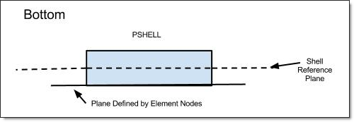
Figure 2: Bottom option in ZOFFS
Note that when ZOFFS is used, both MID1 and MID2 must be specified on the PSHELL entry referenced by this element (otherwise, singular matrices would result).
Offset is applied to all element matrices (stiffness, mass and geometric stiffness) and to respective element loads (such as gravity). Hence, ZOFFS can be used in all types of analysis and optimization. Automatic offset control is available in composite free-size and sizing optimization where the specified offset values are automatically updated based on thickness changes.
However, while offset is correctly applied in geometric stiffness matrix and hence can be used in linear buckling analysis, caution is advised in interpreting the results. Without offset, a typical simple structure will bifurcate and loose stability “instantly” at the critical load. With offset, though, the loss of stability is gradual and asymptotically reaches a limit load, as shown below in figure (b):
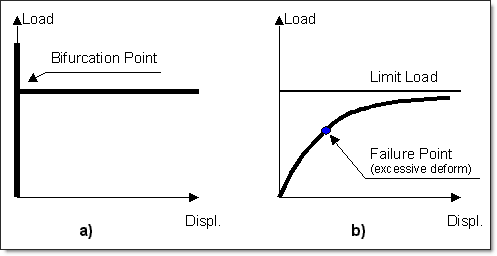
Therefore, the structure with offset can reach excessive deformation before the limit load is reached. The above illustrations apply to linear buckling – in a fully nonlinear limit load simulation, additional instability points may be present on the load path.
| 7. | Stresses and strains are output in the local coordinate system identified by |
| 8. | Size optimization of the property referenced by PID is not possible if Ti values are defined here. If the property referenced by PID is selected as a region for free-size optimization, then any Ti values defined here are ignored. |
| 9. | These 2nd order shell elements do not have normal rotational degrees-of-freedom (often referred to as "drilling stiffness"). No mass is associated with these degrees-of-freedom. If unconstrained, massless mechanisms may occur. It is therefore advisable to use PARAM,AUTOSPC,YES when working with these elements. |
| 10. | This card is represented as a tria6 element in HyperMesh. |
See Also: