NLFE Body Panel - Connectivity Tab

The Connectivity tab allows you to select the sequence of points that define the longitudinal profile of the NLFE Beam or Cable.

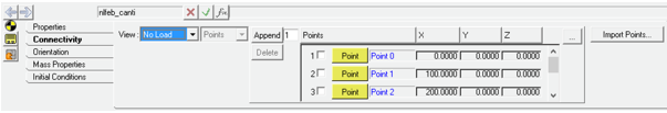
large_deform_body_panel_connectivity_tab_mv

NLFE Body panel - Connectivity tab

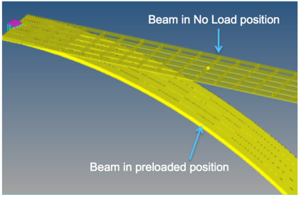
The profile is generally defined as a “No Load” configuration of the beam. This means that the beam modeled in this profile does not have any load on it at the beginning of the simulation. Defining a No Load profile is mandatory.

To define a No Load profile, existing points in the model can be chosen or a .csv file that contains coordinate information for the points can be imported. When the csv file is imported, new points are created using the coordinates information in the file.

There is an option to define a pre-load or loaded configuration. The loaded profile data is different than the no load profile and this difference introduces the pre-load in the body at the beginning of the simulation. Defining a Loaded configuration is optional. If a Loaded configuration is not specified, the body is in an unloaded state at the beginning of the simulation.

The following options are available in the Connectivity tab:

Option	Description
View	Specify the Beam/Cable profile data. The beam profile can be defined for No Load as well as a Loaded configuration (see comments below).
	No Load	Specify the Beam profile as a No Load configuration. The table contains a column of Point collectors to select existing points in the model that form the profile. Alternatively, a csv file containing the point coordinates data can be imported using Import Points button. The following options are available for No Load:
		Append	Enter the number of points to be appended to the Points list and click to add. By default, three rows of point collectors are available.
		Delete	Select the points in the list and click to delete.
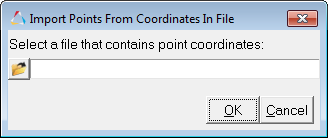
		Import Points	Click to bring up the Import Points From Coordinates In File dialog: The CSV file format is quite intuitive, where each line defines a point. Each line contains three numbers: the X, Y, and Z coordinates of a point. Comment lines begin with a “#”. The example below shows a typical CSV file for a beam that lies initially along the Global X-axis. # Define the nodes for the beam 1.0, 0.0, 0.0 2.0, 0.0, 0.0 3.0, 0.0, 0.0 4.0, 0.0, 0.0 Upon clicking OK, MotionView creates a point entity for each row of values in the csv file and resolves it into the Point collector.
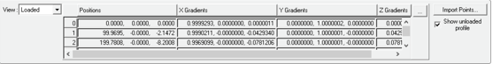
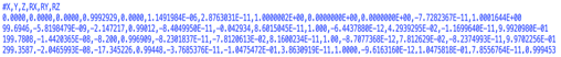
	Loaded	Toggle the View option to Loaded in order to view/define the loaded configuration. Defining a loaded configuration is optional. The loaded configuration consists of Positions, which are three coordinate values. They can be thought of as resulting coordinate values for each profile point defined in the No load configuration in the loaded state. In addition, there are three gradient vectors called as Gradients in each direction – X Gradients, Y Gradients, and Z Gradients. The gradients in a way measure the load at the given position. Refer to Appendix below for more details and to know how a loaded configuration can be obtained.
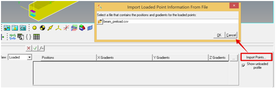
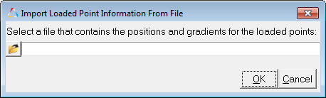
		Import Points	Import a Loaded configuration through a csv file. The format of the csv file required is similar to that of the no load profile, except that the loaded configuration csv file has more columns to accommodate the gradients.

Note

An additional set of constraints is introduced by default at an NLFE grid when a marker (an explicit marker or implicit by means of joints/forces) is associated with the NLFE Body at that grid position. This constraint rigidifies the grid. The constraints are of the form <CONN0 id = “conn_id” gid = “grid_id” conn = “TTTTTT” />. The statement constrains the gradient vector. The first three keywords ‘T’ in the conn attribute represent the constraint on the gradients along X, Y, and Z direction, while the remaining three ‘T’ keywords represent the constraint in the rotational (shear) direction. The form of these constraints can be changed using an environment variable HW_NLFE_CONN_TYPE = ssssss, where s can be either ‘T’ or ‘F’.

Appendix

GRIDs, Position, and Gradients

As mentioned earlier NLFE body is based on a finite element formulation, so, an NLFE Body is represented as a series of elements connected through GRIDs (like node in FE).

A GRID has following attributes and characteristics:

•	Position vector – three Coordinate values in the Body Coordinate System.

•	Gradient vectors – three independent vectors RX, RY, and RZ.

o	A gradient vector is described by three values (similar to a Direction Cosine) in the Body Coordinate System.

•	Gradients of an undeformed GRID are mutually perpendicular forming a right handed coordinate system.

•	Gradients of an undeformed GRID also are unit vectors.

•	Deformation of the GRID is captured by change in length and direction of the gradients.

•	An NLFE GRID has 12 d.o.f.

large_deform_body_panel_conn_tab_beam_example_mv

Beam element (Rod cross section) representation with grid and its gradients

In the figure above, g1 and g2 are the GRIDs of the element with rA and rB being position vectors at end A and B respectively. rxA, ryA, and rzA are the three gradients at end A, while rxB, ryB, and rzB are the three gradients at end B.

The figure below shows gradients of a beam with Bar cross section without any load as well as the same beam, which is loaded under pure tension.

The gradients of the beam without any load are unit vectors and mutually perpendicular, while the beam under tension has its gradients’ magnitude other than 1. A value of more than 1 indicates an increase in the dimension while a value less than one indicates a decrease in the dimension.

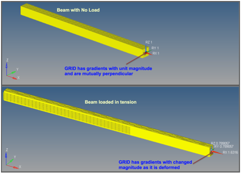
large_deform_body_panel_conn_tab_beam_example2_mv

Gradients of a No Load beam and a Loaded beam in tension

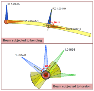
The figure below shows the gradients while in bending as well as torsion. Note that the gradients are no longer perpendicular to each other.

large_deform_body_panel_conn_tab_beam_example3_mv

Generating Position & Gradients for Loaded Configuration

Following process can be followed to generate a CSV file containing the position and gradients for loaded configuration, which can then be imported and saved into MotionView model.

1.	Start with the NLFE Body in a No Load configuration and apply Force/Motion to load the NLFE Body as needed.

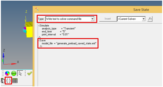
2.	Include the MotionSolve Save command to save the states of the model into an XML file (herein referred as “saved state XML”) after the Simulate command. A template that writes into the solver command section can be used in MotionView.

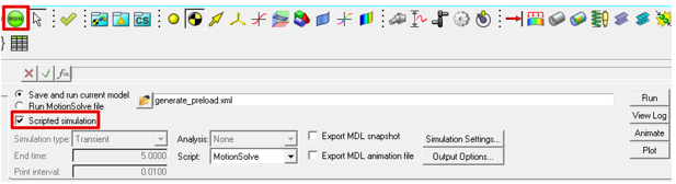
large_deform_body_panel_conn_tab_template_mv

3.	Solve the model. From the MotionView Run panel, use the Scripted simulation option.

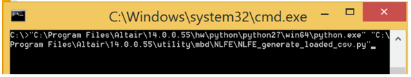
large_deform_body_panel_conn_tab_run_panel_mv

Use a python script “NLFE_generate_loaded_csv.py” available in the Hyperworks install (install_location/utility/mbd/NLFE) to extract the final loaded state of the NLFE Body and save it into a CSV file. The python executable “python.exe” (if not installed separately) can also be found in the Hyperworks install (install_location/hw/python\python27\win64).

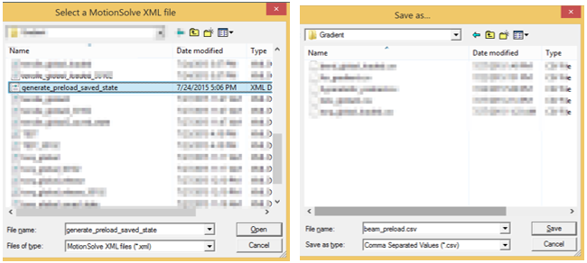
large_deform_body_panel_conn_tab_command_wndw_mv

The script will prompt you to open the saved state XML file and also provide a CSV file name to save the position and gradients information.

large_deform_body_panel_conn_tab_save_as_dialog_mv

5.	Once the CSV file is saved, import it into MotionView using the Import Points option available in the Loaded View of the NLFE Connectivity tab.

large_deform_body_panel_conn_tab_import_points_mv

Upon importing the loaded configuration, the display of the NLFE Body in graphics area would change. The NLFE Body loaded configuration gets the prominent display with solid implicit graphics while the no load configuration will be shown in a wireframe featured mode.

large_deform_body_panel_conn_tab_beam_no_load_preload_ex_mv