Title
Law characterization
|
|
Number
11.1
|
Brief Description
Elasto-plastic material law characterization using a tensile test.
|
Keywords
| • | Johnson-Cook elasto-plastic model (/MAT/LAW2) |
| • | Necking point, damage model, maximum stress, and failure plastic strain |
|
RADIOSS Options
| • | Boundary conditions (/BCS) |
| • | Material definition (/MAT) |
|
Compared to / Validation Method
|
Input File
Law_2_Johnson_Cook: <install_directory>/demos/hwsolvers/radioss/11_Tensile_test/Law_2_Johnson-Cook/.../TENSIL2*
Law 27_Damage: <install_directory>/demos/hwsolvers/radioss/11_Tensile_test/Law_27_Damage/DAMAGE*
Law_36_Tabulated: <install_directory>/demos/hwsolvers/radioss/11_Tensile_test/Law_36_Tabulated/TENSI36*
|
Technical / Theoretical Level
Advanced
|
Overview
Aim of the Problem
It is not always easy to characterize a material law for transient analysis using the experimental results of a tensile test. The purpose of this example is to introduce a method for characterizing the most commonly used RADIOSS material laws for modeling elasto-plastic material. The use of "engineering” or "true” stress-strain curves is pointed out. Damage and failure models are also introduced to better fit the experimental response.
Apart from the experimental results, the modeling of the strain rate effect on stress will be considered at the end of this example using a sensitivity study on a set of parameters for Johnson-Cook’s model.
Physical Problem Description
Traction is applied to an object. A quarter of the object is modeled using symmetrical conditions. The material to be characterized is 6063 T7 Aluminum. A velocity is imposed at the left-end.
Units: mm, ms, g, N, MPa.
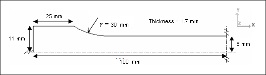
Fig 1: Geometry of the tensile object (One quarter of the object is modeled).
The material undergoes isotropic elasto-plastic behavior which can be reproduced by a Johnson-Cook model with or without damage (/MAT/LAW27 and /MAT/LAW2, respectively). The tabulated material law (/MAT/LAW36) is also studied.
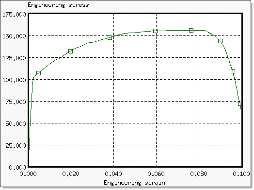
Fig 2: Experimental results of the tensile test: engineering stress vs. engineering strain.
Analysis, Assumptions and Modeling Description
Modeling Methodology
The average element size is about 2 mm in the mesh (Fig 3). There are 201 4-node shells and one 3-node shell.
The shell properties are:
| • | 5 integration points (progressive plastification). |
| • | Belytschko elasto-plastic hourglass formulation (Ishell = 3). |
| • | Iterative plasticity for plane stress (Newton-Raphson method; Iplas = 1). |
| • | Thickness changes are taken into account in stress computation (Ithick = 1). |
| • | Initial thickness is uniform, equal to 1.7 mm. |
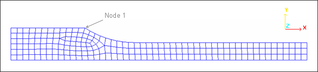
Fig 3: Mesh of the object.
| • | Node number 54 was renamed "Node 1" to be compliant with the Time History. |
For node 54, only displacements in the x-direction (variable DX) are saved.
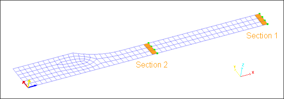
Fig 4: Sections saved for Time History.
For both sections, the variables FN and FTX, are saved; thus the following variables will be available in /TH/SECTIO: FNX, FNY, FNZ (saved using "FN"), and FTX.
Engineering strains will be obtained by dividing the displacement of node 1 with the distance up to the symmetry axis (75 mm). Engineering stresses will be obtained by dividing the force through section 1 with its initial surface (10.5 mm2). Therefore, the results shown correspond to the engineering stress as a function of the engineering strain, equivalent to the force variation compared to displacement (similar curve shape).
RADIOSS Options Used
An imposed velocity of -1.0 m/s in the x-direction is applied to the nodes, shown below (abscissa less than or equal to 25 mm). The displacement is proportional to time.
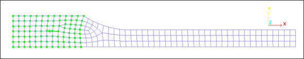
Fig 5: Imposed velocities
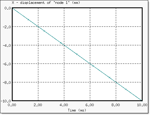
Fig 6: Variation of node 1 x-displacement in relation to time.
Only one quarter of the object is modeled to limit the model size and to eliminate the rigid body motions. Symmetry planes are defined along axis x = 100 mm and axis y = 0. Two boundary conditions cannot be applied to the same node 13 (corner).
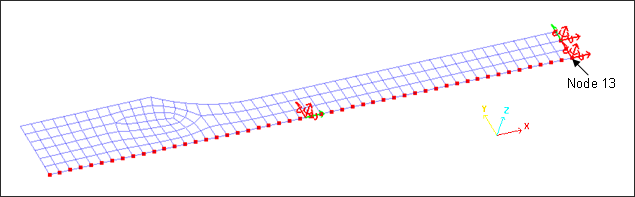
Fig 7: Boundary conditions
The lower side is fixed in Y and Z translations and X, Y, and Z rotations.
The right side is fixed in X and Z translations and X, Y, and Z rotations; the node in the corner is completely fixed.
Characterization of the Material Law
There are two steps to characterize the material law:
| • | Transform the engineering stress versus engineering strain curve into a true stress versus true strain curve (this step applies to any material law). |
| • | Extract the main parameters from the true stress versus true strain curve, to define the material law (Johnson-Cook law and material coefficients for /MAT/LAW2 or the yield curve definition for /MAT/LAW36). |
- True stress/true strain curve
Engineering strains are computed using the following relationship:

And true strains are computed with the relationship:
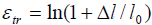
Both strains, therefore, are linked together by:
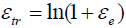
Engineering stresses are measured by dividing the force through one section with the initial section. True stresses are measured by dividing the force with the true deformed section:
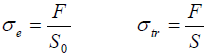
Thus, to compute true stresses, the surface variation must be taken into account. Assuming that Poisson’s coefficient is 0.5 during plastic deformation, the true surface in mono-axial traction is:
Thus, the relationship between true and engineering stresses is:
Characterization of the Material Law
The characterization will be made for /MAT/LAW2 (Johnson-Cook elasto-plastic), /MAT/LAW27 (elasto-plastic with damaged model) and /MAT/LAW36 (tabulated elasto-plastic). For each of the material laws, the yield stress and Young’s modulus are determined from the curve.
The plastic strain can be defined as:
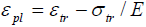
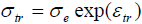
An important point to be characterized on the curve is the necking point, where the slope of the force versus the displacement curve is equal to 0, and where the following relationships apply:
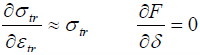
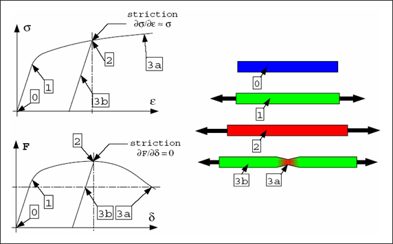
Fig 8: Guidelines for necking point.
Table 1: Equations used for analysis
Material Property
|
Generic Equation
|
Engineering stress
|

|
Engineering strain
|
|
True stress
|
|
True strain
|
|
True strain rate
|

|
Simulation Results and Conclusions
Experimental Results
An experiment designed by the "Norwegian Institute of Technology" as part of an EC-financed program, "Calibration of Impact Rigs for Dynamic Crash Testing" is used. The following curve was obtained from the experiment:
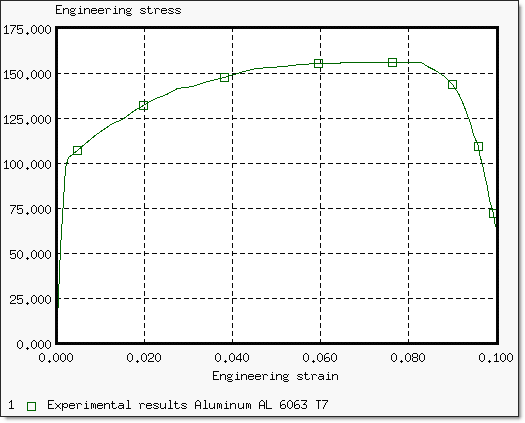
Fig 9: Engineering stress versus engineering strain curve (experimental data).
It is estimated that the necking point occurs between 6% and 8% (engineering strain). After analyzing the experimental data, the first point satisfying the necking condition is at 6.68%.
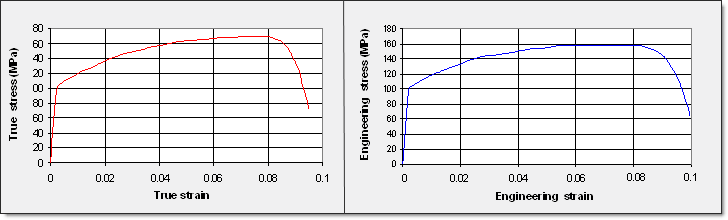
Fig 10: Comparison between engineering and true curves (from experimental data).
Engineering formulation is converted into true formulation using the relationship:
The true stress curve is higher than the engineering stress curve, as it takes into account the decrease in the objects cross-section.
Law 2: Elasto-plastic Material Law Using the Johnson-Cook Model
Johnson-Cook Material Coefficients
The stress versus plastic strain law is: (Johnson-Cook model)
where, a is the yield stress and is read from the experimental curve and then converted into true stress.
To compute b and n, two states are needed. This leads to the following formulas for b and n:
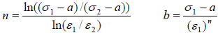
The first point is chosen at the necking point, then b and n are computed for each other point of the curve and averaged out since the results tend to differ depending on the point chosen.
Characterization up to the Necking Point
The first stage when determining the material model is to obtain Johnson-Cook’s coefficients. Neither the maximum stress, nor the failure plastic strain effects are taken into account here (set at zero).
The values of coefficients are chosen so that the model adapts to the test data.
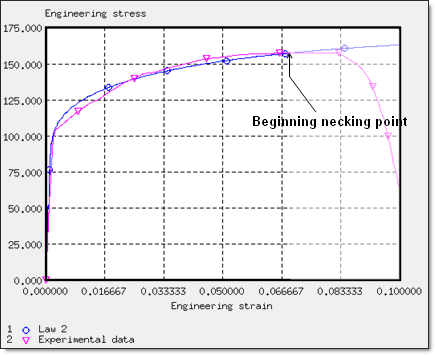
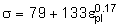
Fig 11: Variation of the engineering stress/strain according to Johnson-Cook’s model adapted to the test.
The material coefficients used for Law 2 are:
| Initial density: 2.7x10⁻³ g/mm3 | Yield stress: 90.27 MPa |
| Poisson’s ratio: 0.33 | Hardening parameter: 223.14 MPa |
| Young’s modulus: 60400 MPa | Hardening exponent: 0.375 |
Figure 12 compares the yield curve defined using the Johnson-Cook model with the one extracted from experimental data.
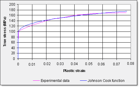
Fig 12: Yield curves Johnson-Cook model 1
The true stress – true strain relationship can be described by:
The engineering stress deviations between experiment and simulation are described in the table below:
Engineering strain
|
0.01
|
0.02
|
0.03
|
0.04
|
0.05
|
0.06
|
0.067
|
Deviation
|
7.9%
|
4.8%
|
1.8%
|
1.1%
|
1%
|
1.8%
|
2.9%
|
Comparison is performed up to the necking point (engineering strain = 6.68%) because after this state, a rapid decrease in the engineering stresses occurs in the object. The rupture sequence is simulated in the following paragraphs. Results using Law 2 remain within 8% of the experimental curve.
The curve could be improved by slightly adjusting some of the values. The purpose of this test is to propose a method for deducing material law parameters using a tensile test.
Beginning of the Necking Point
Necking Point Simulation
The Johnson-Cook model previously defined corresponds to the experimental results up to the necking point. However, the slope of the numerical response does not enable the necking point to start at the strain value observed experimentally.
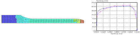
The necking point is characterized by the slope value of the true stress versus the true strain curve, which must be approximately equal to the true stress. The necking point numerically appears by continuing simulation until the condition on the slope is observed.
The results are obtained using the Johnson-Cook model 1:
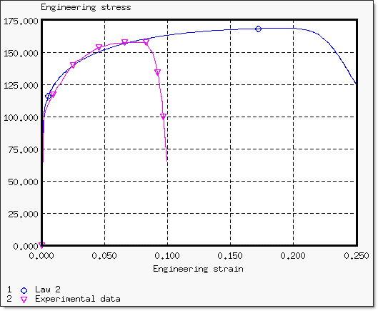
Fig 13: Beginning of the necking point using only the first coefficients of the Johnson-Cook model (a, b and n).
Fig 14: True stress versus true strain curve up to the beginning of the necking point.
The necking point can be simulated, either by adjusting the Johnson-Cook coefficients to obtain an accurate slope, or by compelling curve with a maximum stress.
Simulation of the Slope Near the Necking Point
By implementing an energy approach, the hardening curve can be modified to achieve an engineering curve which resembles a horizontal asymptote near the necking point with the purpose of simulating the behavior of the curve as observed in the test.
The Johnson-Cook coefficients used to describe the physical slope are:
Yield stress: 79 MPa
Hardening parameter: 133 MPa
Hardening exponent: 0.17
For this model, the new true stress/true strain relationship is:
 | (Johnson-Cook model 2) |
The results obtained with those coefficients are provided below.
Figure 15 compares the Johnson-Cook model 3 with the experiment:
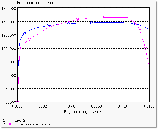
Fig 15: Adjusted engineering stress/strain curve to model the beginning of the necking point.
The shape of the yield curve versus the experimental data is depicted in Fig 16.
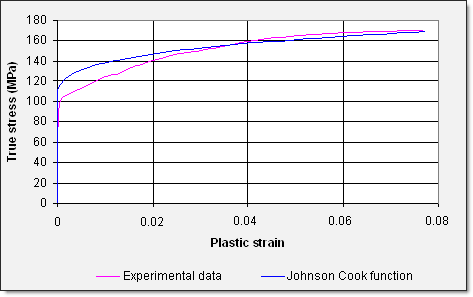
Fig 16: Yield curves.
The necking point is defined as  .
.
This condition is characterized by the intersection of the true stress versus the true strain curve with its derivate.
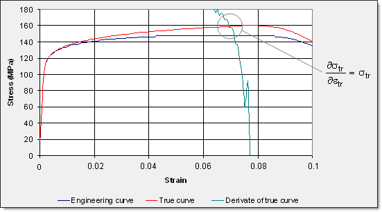
Fig 17: Superposition of engineering curve and true curve with its derivate.
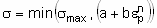
Beginning of the Necking Point Using a Maximum Stress Limit,  max
max
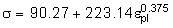
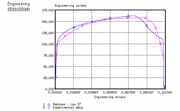
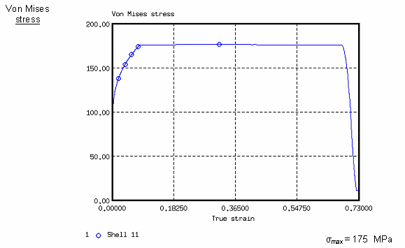
For this test, the Johnson-Cook coefficients input are those set in characterization up to the necking point, the failure effect not being taken into account (the failure plastic strain is set to zero). The beginning of the necking point is set using the choice of a maximum stress value. In comparison to the experimental results (see Fig 10), the necking point is well defined for a maximum stress set at 175 MPa. The limit in stress appears on the von Mises stress versus true strain curve on elements where the necking point occurs.
The maximum true stress manages the beginning of the necking, as shown below:
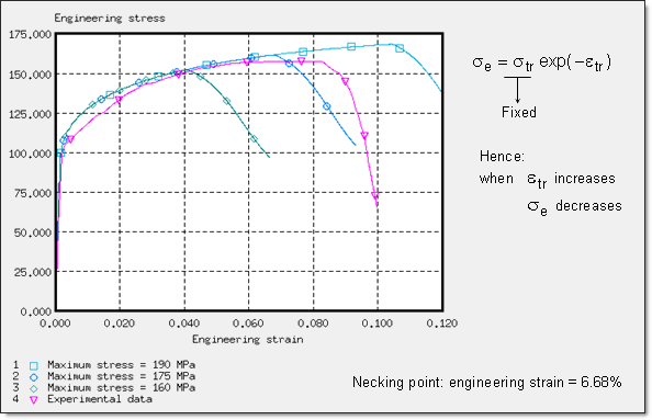
Fig 18: Engineering stress versus engineering strain; necking point characterization
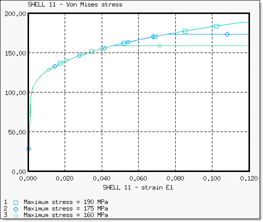
Fig 19: Variation of the von Mises stress with the true strain from shell 11.
Maximum stress  max is reached for von Mises stress on shells where the necking begins. To avoid overly-high stresses after the necking point, a maximum stress factor must be set approximately equal to the true necking point stress.
The following curves show the evolution of the von Mises stress versus the true strain shell at two characteristic locations of the object (3b and 3a in Fig 20):
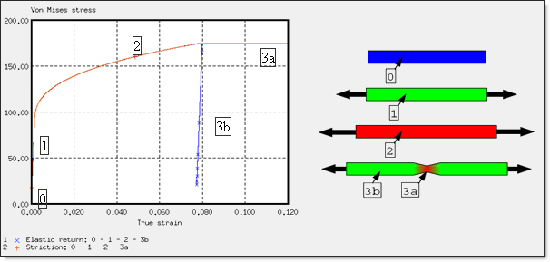
Fig 20: von Mises stress curve with a maximum stress limit.
The beginning of the necking point is observed following the point where the stress is equal to stress versus strain derivate  .
.
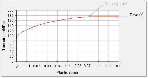
Fig 21: Yield curve with maximum stress.
The yield curve is described by:
The derivate of the stress is very sensitive and strongly depends on the yield curve definition. Thus, introducing the necking point into the simulation is very delicate (a small change can result in many variations). The necking point should first begin on a given element for numerical reasons. The preferred beginning of necking is addressed below.
Preferred Beginning of the Necking Point
Experimentally, the beginning of the necking point can appear anywhere on the object. The beginning of the necking point should preferably be located on the right end elements in order to propose a methodology for this quasi-static test. If the model only uses a quarter part of the object, the necking point is found on elements 30, 125 and 78.
The beginning of the necking point is physically and numerically sensitive and can be initiated on the right elements by changing a few of the coordinates along the Y-axis of the node in the right corner (node 16) in order to decrease the cross-section and privilege the necking point in this zone. Changing the node position by 0.01 mm is enough for achieving the preferential beginning of the necking point.
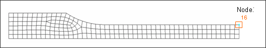
Fig 22: Node 16 to be moved.
A second approach also enables the necking point to be triggered on the right end side by defining an extra part, including shells 3, 11 and 4 by using a maximum stress slightly lower than the remaining part, in order to initiate the necking point locally since the necking point stress is first reached in the elements having the lowest maximum stress value, that is shells 3, 11 and 4. This method, based on material properties, is quite appropriate for demonstrating the characterization of a material law and will thus be used in the continuation of the example.
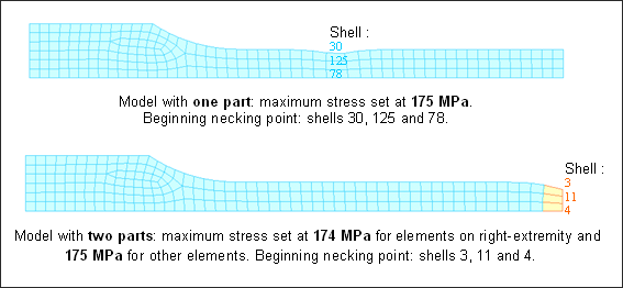
Fig 23: Localization of the beginning of the necking point according to the models using max.
The material is described as Johnson-Cook model 1:
max = 174 / 175 MPa
The following curves indicate the variation of the engineering stress versus the engineering strain according to the beginning of the necking point zone and in comparison to the experiment.
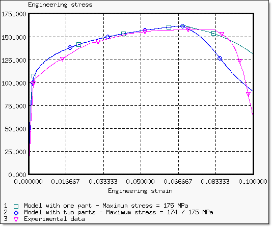
Fig 24: Engineering stress/strain curve for each starting necking point location.
There is a fast decrease in the engineering stress after the right-end necking point. The necking point, due to the boundary conditions of the y-symmetry plane (y-translation DOF released), becomes more pronounced.
The variations in the section where the necking point is found are quite similar up to the necking point. After such point, there is a sharp surface decrease for the right-end necking point, contrary to the second case where the surface decrease is more moderate.
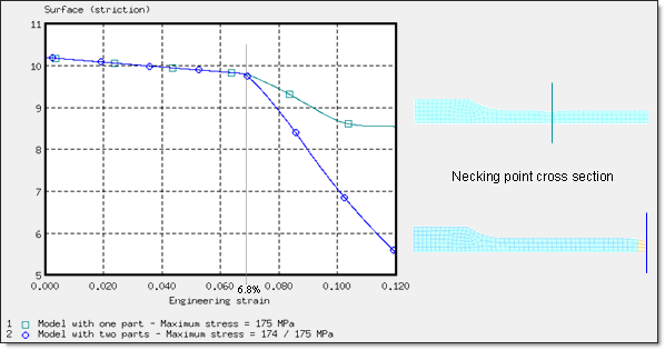
Fig 25: Variation of cross section (necking point zone).
Improvement of the Elements’ Contribution During the Necking Point Sequence
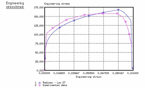
In order to simulate physically the contribution of each element in the necking point, it is advisable to adjust the curve by varying the Johnson-Cook coefficients in order to increase the intensity of stress at the necking point. The main result is no longer the variation of the stress/strain curve but rather the surface under the curve which characterizes the energy dissipated during the test. This energy-based approach is relevant for crash tests since the final assessment is often more significant than how it was achieved.

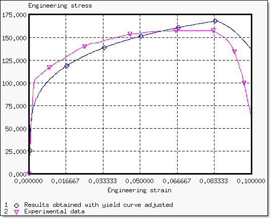
Fig 26: Engineering stress/strain curve obtained using adjusted Johnson-Cook coefficients.
The following graph compares the new yield curve with experimental data:
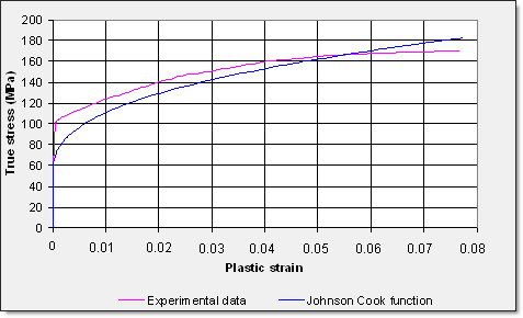
Fig 27: Yield curves.
Material is described in the the Johnson-Cook coefficients are:
Johnson-Cook Model 3:
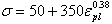 (true stress/strain)
Yield stress = 50 MPa
Hardening parameter = 350 MPa
Hardening exponent = 0.38
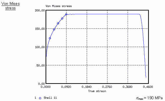
Maximum stress is set to 189 or 190 MPa (according to the parts)
The results of adjustment to the Johnson-Cook coefficients are depicted below:
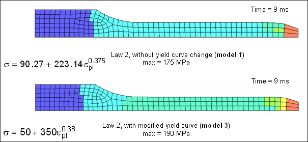
Fig 28: Shell contribution during the necking point sequence (von Mises stress).
As the necking point progresses, more physical results are obtained due to the new input data of the material law coefficients having a better element contribution.
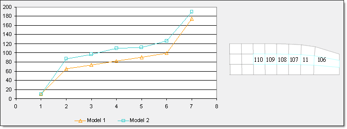
Fig 29: Variation of the von Mises stress on elements 110, 109, 108, 107, 11 and 106.
Damage Modeling with Plastic Strain Failure
The elasto-plastic model of Johnson-Cook is used until failure, which is simulated using a plastic strain failure option. The element is deleted if the plastic strain reaches a user-defined value  max. This damage model shows good stability. A maximum plastic strain is defined for each Johnson-Cook model:
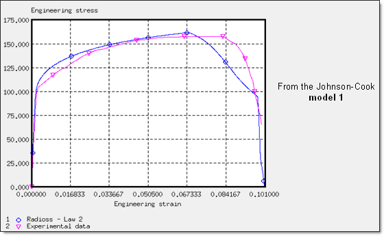
Fig 30: max = 75% ; yield curve close to experimental data:
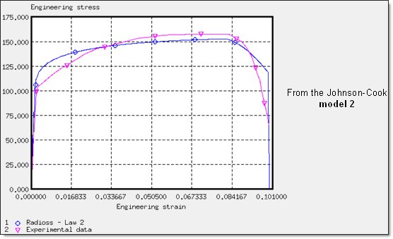
Fig 31: max = 47% ; yield curve adjusted with respect to lower stresses: 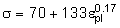 .
.
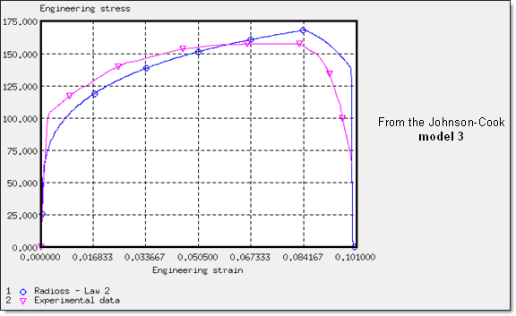
Fig 32: max = 40% ; yield curve adjusted with respect to high stresses: 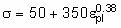 .
.
Failure is reached for relatively high true strains.
Law 27: Elasto-plastic Material Law with Model Damage
Law 27 is used to simulate material damage following a Johnson-Cook plasticity law. Thus, model damage is associated with the previous law in order to take account of failure.
The damage parameters are:
| • | Tensile rupture strain t1: damage starts if the highest principal strain reaches this tension value. |
| • | Maximum strain m1: the element is damaged if the highest principal strain is above the tension value. The element is not deleted. |
| • | Maximum damage factors max: this value should be kept at its default value (0.999). |
| • | Failure strain f1: the element is deleted if the highest principal strain reaches the tension value. |
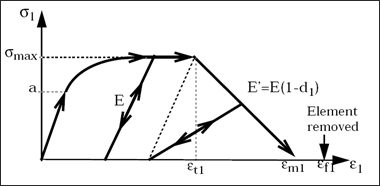
Fig 33: Stress/strain curve for damage affected material.
The following graphs display the results obtained using the material coefficients of two previous Johnson-Cook models. Damage parameters complete those models.
Damage Model A
|
|
|
Damage model: t1 = 0.16 ; m1 = 0.72 ; dmax = 0.999 ; f = 1 ; max = 16
|
Johnson-Cook model:
|
Damage Model B
|
|
|
Damage model: t1 = 0.16 ; m1 = 0.45 ; dmax = 0.999 ; f = 1 ; max = 16
|
Johnson-Cook model:
|
Law 36: Tabulated Elasto-plastic Law
This is a tabulated law; therefore, the true stress versus plastic strain function can be directly used. The rupture phase can be simulated by adding points to this hardening function.
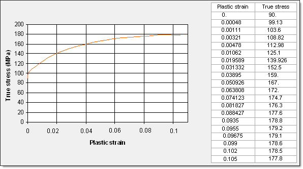
Fig 34: Hardening function defined in law 36 to obtain the results below.
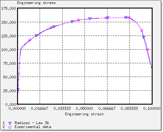
Fig 35: Results obtained with tabulated law 36.
The hardening curve has to be defined with precision around the necking point while the decrease of the curve is very sensitive to its adjustment. In order to improve the modeling of the necking point, two points can be interpolated, one "just before" the necking point, and one "just after" with the slope between those two points equal to the necking point stress.


