|
»Click here to display Table of Contents«
|

Example 25 - Spring-back |

|

|

|

|
|
Example 25 - Spring-back |
|
|
|

|
|
»Click here to display Table of Contents«
|
Example 25 - Spring-back |
|
|
|
|
|
Example 25 - Spring-back |
|
|
|
|
The spring-back simulation of sheet metal bent into a hat-shape is studied. The problem is one of the famous tests from the Numisheet’93. As spring-back is generally a quasi-static unloading, the use of the RADIOSS implicit solver is justified. The RADIOSS explicit solver is also used to compare the methods’ efficiency. However, for the stamping phase only the explicit solver is used, as the forming process is highly dynamic.
The example illustrates how to link up the explicit computations. It highlights the efficiency of the implicit solver for the spring-back simulation.
TitleSpring-back |
|
||||||||||||
Number25.1 |
|||||||||||||
Brief DescriptionAn explicit stamping simulation is followed by a spring-back analysis using implicit or explicit solvers for stress relaxation. Results are compared with a reference. |
|||||||||||||
Keywords
|
|||||||||||||
RADIOSS Options
|
|||||||||||||
Compared to / Validation Method
|
|||||||||||||
Input FileExplicit spring-back: <install_directory>/demos/hwsolvers/radioss/25_Spring-back/Explicit_spring-back/DBEND_44* Implicit spring-back: <install_directory>/demos/hwsolvers/radioss/25_Spring-back/Implicit_spring-back/DBEND_44* |
|||||||||||||
Technical / Theoretical LevelAdvanced |
|||||||||||||
This example deals with the numerical simulation of a stamping process, including the spring-back. This refers to one of the sheet metal stamping tests "2D Draw Bending" indicated in Numisheet’93. The final shape of the formed sheet metal, after releasing all constraints on the blank sheet is studied. During the spring-back simulation, an explicit-to-implicit sequential solution method is used, where a dynamic forming process using the explicit solver is used first, followed by an implicit modeling of the spring-back deformations by statically removing the stamping stress.
Thus, two analyses are performed in order to compare the performances and the accuracy of results:
| • | Explicit stamping and implicit spring-back simulations |
| • | Explicit stamping and explicit spring-back simulations (using dynamic relaxation) |
The spring-back simulation of the forming sheet metal uses an elasto-plastic nonlinear approach. The implicit input options and the incremental strategy used are described in the modeling section.
A numerical simulation of stamping is performed up to 960 ms. Spring-back computation is carried out from 960 ms to 1000 ms for implicit (static approach) and to 6000 ms for explicit (quasi-static approach).
A standard stamping operation is studied. The stamping tools include a punch, a die and a blank holder.
Units: mm, ms, g, N, MPa.
A load F of 1225 N is vertically applied on the blank holder in order to flatten the sheet metal against the die. The load is removed before spring-back simulation.
The sheet metal stamping operation is managed using a variable imposed velocity applied on the punch with a maximum set to 0.1 ms-1. The tools are withdrawn after the stamping phase in order to enable the spring-back to be observed.
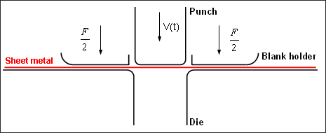
Fig 1: Description of the problem.
The main geometrical dimensions of parts are:
| • | Radius of die’s corners: 5 mm |
| • | Radius of punch’s corners: 5 mm |
| • | Width of punch: 50.4 mm |
| • | Sheet metal dimensions: 35 mm x 175 mm |
The thickness of the sheet metal is defined at 0.74 mm. The Coulomb friction coefficient between the sheet metal and the die is defined at 0.129.
The stamping tools’ material undergoes a linear law using the following properties:
| • | Initial density: 8x10⁻³ g/mm3 |
| • | Young modulus: 206000 MPa |
| • | Poisson ratio: 0.3 |
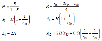
The material of the sheet metal under the roller has distinct characteristics of anisotropy. Its anisotropic elasto-plastic behavior can be reproduced by a Hill model (/MAT/LAW43). This law can be considered as a generalization of the von Mises yield criteria for anisotropic yield behavior.
The yield stress is defined according to a user function and the yield stress is compared to equivalent stress:
![]()
The Ai coefficients are determined using Lankford’s anisotropy parameters range. Angles for Lankford parameters are defined according to orthotropic direction 1.
A hardening coefficient is used to describe the hardening model as full isotropic (value set to 0) or based on the Prager-Ziegler kinematic model (value set to 1). Hardening can be interpolated between the two models, if the coefficient value is between 0 and 1.
The material parameters are:
| • | Initial density: 8x10⁻³ g/mm3 |
| • | Young modulus: 206000 MPa |
| • | Poisson ratio: 0.3 |
| • | Lankford 0 degrees: r00= 1.73 |
| • | Lankford 45 degrees: r45 = 1.34 |
| • | Lankford 90 degrees: r90= 2.24 |
The yield curve used is shown in the diagram below. Failure is not taken into account.
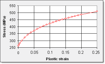
Fig 2: User’s yield function.
Taking symmetry into account, only a quarter of the structure is modeled. The symmetry plane is along axis y = 17.5 mm and x = 0 mm.
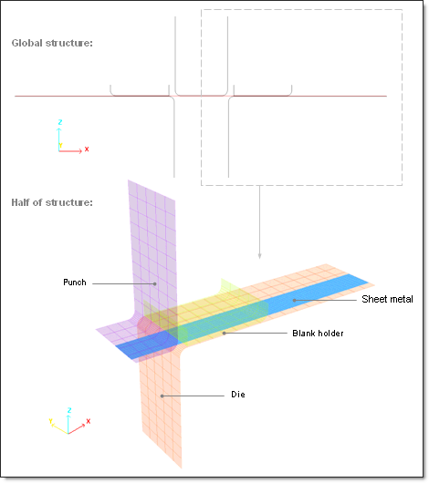
Fig 3: Finite mesh elements of the problem studied.
The punch is shown in purple, the blank holder in green and the die in red. The sheet metal (blue) is modeled using 4-node shell elements.
The sheet metal is discretized by a non-regular mesh and a fine mesh is used for parts to be plastically deformed. The smallest size of the shell element is 1.5 mm.
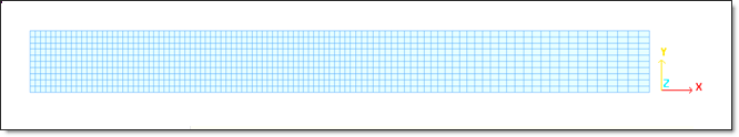
Fig 4: Progressive mesh of the sheet metal.
In order to achieve accurate simulation results, the QEPH shell element formulation is used in explicit and implicit analyses. A Lagrangian formulation is adopted.
In accordance with the elasto-plastic Hill model for the material law, the sheet metal is described by the shell elements using the orthotropic property (Type 9). The shell characteristics are:
| • | Five integration points (progressive plastification) |
| • | Interactive plasticity with three Newton iterations (Iplas = 1) |
| • | Thickness changes are taken into account in stress computation (Ithick = 1) |
| • | Initial thickness is uniform, equal to 0.74 mm |
| • | Orthotropy angle: 0 degree |
| • | Reference vector: (1 0 0) |
The input components of the reference vector ![]() are used to define direction 1 of the local coordinate system of orthotropy. The orthotropy angle, in degrees defines the angle between direction 1 of the orthotropy and the projection of the vector
are used to define direction 1 of the local coordinate system of orthotropy. The orthotropy angle, in degrees defines the angle between direction 1 of the orthotropy and the projection of the vector ![]() on the shell.
on the shell.
Three type 7 interfaces using the Penalty method are employed to model contacts between the stamping tools and the sheet metal. The parameters defining the contact are:
| • | Coulomb friction: 0.129 |
| • | Gap: 0.37 |
| • | Critical damping coefficient on interface stiffness: 1 |
| • | Critical damping coefficient on interface friction: 1 (default) |
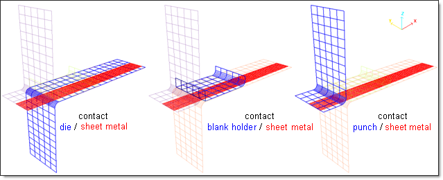
Fig 5: Contact modeling using a type 7 interface considered with the Penalty method (master/slave sides).
In the implicit approach, the contact using the Penalty method with fictional springs is stored in a separate stiffness matrix to the main one. Therefore, supplementary memory is needed and information of the second contact stiffness will be printed when contact is active.
Critical damping coefficients (inputs) description:
| • | The normal force computation is indicated by: |
![]()
Where,
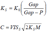
K0 is the initial interface spring stiffness
VISCS is the critical damping coefficient on interface stiffness (default value: 0.05)
| • | The tangential force computation is indicated by: |
Ft = min(Fric * Fn, Fad )
where:
Fad = Ct Vt is the adhesion force
![]()
VISf is the critical damping coefficient on interface friction (default value: 1)
For spring-back computation by implicit, the removing of the stamping tools is taken into account by deleting all interfaces using the input option in the second *_0002.rad Engine file as follows:
/DEL/INTER
1 2 3 " Interfaces ID 1, 2 and 3 are deleted.
Simulation deals with:
| 1. | Stamping simulation by explicit: from the beginning up to 960 ms. |
| 2. | Spring-back simulation: |
| • | using explicit (dynamic approach): from 960 ms to 6000 ms: |
| - | From 960 ms to 2000 ms: Stamping tools are slowly withdrawn because the quasi-static analysis requires dynamic effects to be minimized during spring-back. Thus, the interfaces are not deleted. Options are defined in the *_0002.rad Engine file. |
| - | From 2000 ms to 6000 ms: A dynamic relaxation (/DYREL) is activated in the *_0003.rad Engine file in order to converge towards quasi-static equilibrium. |
| • | using implicit (static approach): from 960 ms to 1000 ms: |
| - | The input implicit options are added in the *_0002.rad Engine file. Stress relaxation is activated using the /IMPL/SPRBACK keyword. All interfaces are deleted and specific boundary conditions are added on the stamping tools. Tools are not withdrawn. |
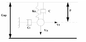
In the simulation, the tools are modeled using rigid bodies (/RBODY) as shown in Fig 6.
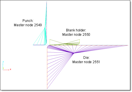
Fig 6: Modeling of the stamping tools as rigid elements.
An automatic master node is chosen. The center of gravity is computed using the master and slave node coordinates and the master node is moved to the center of gravity where is placed mass and inertia (ICoG is set to 1). No mass or inertia are added to the rigid bodies.
A quarter of the structure is modeled in order to limit the model size and to eliminate rigid body modes for implicit computation. Symmetry planes are defined along the y axis = 0.
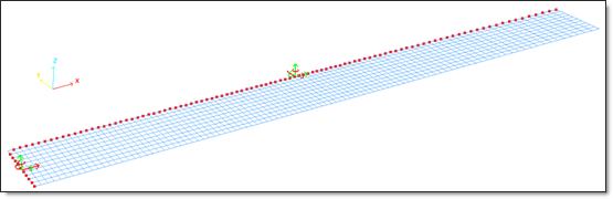
Fig 7: Boundary conditions (/BCS) on the sheet metal according to the symmetries.
The nodes on the longitudinal plane are fixed in the Y translation and X, Z rotations.
For the other symmetry plane, the nodes are fixed in the X translation and Y, Z rotations.
Stamping tools are restricted to moving only along the Z-axis. The boundary conditions are applied on the master nodes of the rigid bodies, including the parts (Fig 7).
For the numerical simulation of the implicit spring-back, additional conditions must be added in the *_0002.rad Engine file in order to remove the rigid body modes that are not permitted in the implicit approach. The stamping tools are fully fixed (X, Y, Z translations and X, Y, Z rotations). The translation of the ID 427 node is fixed along the Z-axis allowing the sheet metal to move towards the final shape without rigid body mode.
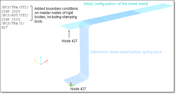
Fig 8: Added boundary conditions on the 427 node for implicit spring-back.
Imposed velocities are applied on the stamping tools via the master nodes of the rigid bodies. The velocity of the punch is controlled by a specific input curve, as shown in Figures 9 and 10. During implicit spring-back, all velocities are set to zero. Explicit spring-back computation up to 6000 ms necessitates imposed velocities on tools in order to withdraw them as of 1000 ms.
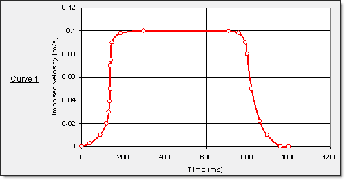
Fig 9: Imposed velocity on punch via the rigid body’s master node.
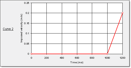
Fig 10: Imposed velocity on die and blank holder via the rigid bodies’ master node.
" Punch part …………… Curve 1, scale factor set to -1.
" Die part ………………. Curve 2, scale factor set to 1.
" Blank holder part ……. Curve 2, scale factor set to -1.
The stamping is performed by explicit simulation up to 960 ms using Curve 1. The implicit simulation is carried out only for the spring-back stage from 960 ms to 1000 ms. Curve 2, therefore, is only defined for explicit spring-back simulation.
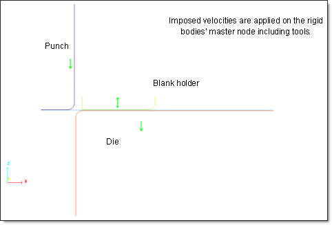
Fig 11: Imposed velocities on tools in two phases: stamping then tools removing.
Considering the symmetries, a constant concentrated load of 612.5 N is vertically applied on the blank holder via the master node of the rigid body. The load is set to zero from 960 ms before studying the spring-back.
Implicit spring-back analysis is launched using /IMPL/SPRBACK.
The nonlinear implicit parameters used are:
Implicit type: |
Static nonlinear |
Nonlinear solver: |
Modified Newton |
Tolerance: |
0.025 |
Update of stiffness matrix: |
2 iterations maximum |
Time step control method: |
Norm displacement (arc-length) |
Initial time step: |
0.08 ms |
Minimum time step: |
10-5 ms |
Maximum time step: |
no |
Desired convergence iteration number: |
6 |
Maximum convergence iteration number: |
20 |
Decreasing time step factor: |
0.67 |
Maximum increasing time step scale factor: |
0.0 |
Arc-length: |
Automatic computation |
Spring-back option: |
Activated |
A solver method is required to resolve Ax=b in each iteration of the nonlinear cycle. It is defined using /IMPL/SOLVER.
Linear solver: |
Direct solver MUMPS |
Precondition methods: |
Factored approximate inverse |
Maximum iterations number: |
System dimension (NDOF) |
Stop criteria: |
Relative residual on force |
Tolerance for stop criteria: |
Machine precision |
The input implicit options added in the *_0002.rad Engine file are:
Printout frequency for nonlinear iteration |
|
/IMPL/NONLIN/1 |
Static nonlinear computation |
/IMPL/SOLVER/2 |
Solver method (solve Ax=b) |
/IMPL/DTINI |
Initial time step determines initial loading increment |
/IMPL/DT/STOP |
Min-Max values for time step |
/IMPL/DT/2 |
Time step control method 2 - Arc-length+Line-search will be used |
Spring-back computation (stress relaxation) |
Refer to RADIOSS Starter Input for more details about implicit options.
Explicit spring-back analysis uses the dynamic relaxation in the *_0003.rad Engine file from 2000 ms.
The explicit time integration scheme starts with nodal acceleration computation. It is efficient for the simulation of dynamic loading. However, a quasi-static simulation via a dynamic resolution method is needed to minimize the dynamic effects for converging towards static equilibrium, the final shape achieved after spring-back.
The dynamic effect is damped by introducing a diagonal damping matrix proportional to mass matrix in the dynamic equation.
![]()
![]()
where, ![]() is the relaxation value which has a recommended default value 1, and T is the period to be damped (less than or equal to the highest period of the system).
is the relaxation value which has a recommended default value 1, and T is the period to be damped (less than or equal to the highest period of the system).
The inputs of the relaxation dynamics are:
| • | Relaxation factor: 1 |
| • | Period to be damped: 1000 ms |
This option is activated using the /DYREL keyword (inputs: ![]() and T).
and T).
In the metal stamping operation, the highly nonlinear deformation processes tend to generate a large amount of elastic strain energy in the metal material in addition to some of the plastic deformed areas. The internal energy, which is stored in the sheet metal during stamping, is subsequently released once the stamping pressure has been removed. This energy released is the driving force of the spring-back in the sheet metal forming process. Therefore, the spring-back deformation for sheet metal forming is mainly due to the amount of elastic energy stored in the part while it is being plastically deformed.
The material density has been multiplied by 10,000 to obtain a reasonable computation time using explicit simulations. An additional time period is also required for slowly withdrawing the tools, prior to the explicit spring-back simulation in order to achieve a good result. Thus, explicit stamping takes longer than stamping followed by implicit spring-back computation.
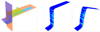
Figure 12 shows the deformed configurations using implicit simulation. The symmetrical part is added.
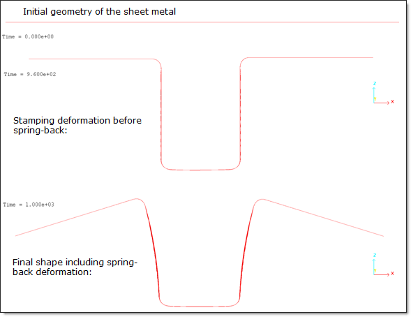
Fig 12: Deformed sheet metal before and after spring-back (implicit spring-back).
Stamping is performed from the beginning up to 960 ms. The final shape after the spring-back process is achieved after 1000 ms using the implicit solver and after 6000 ms using the explicit solver.
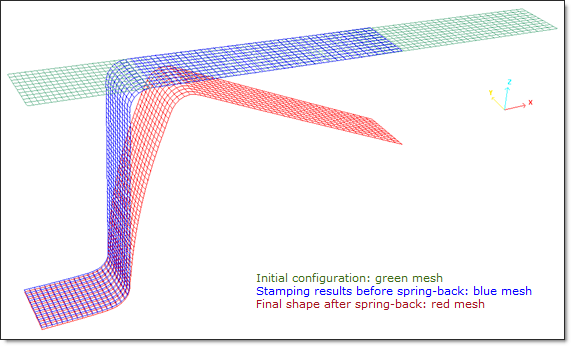
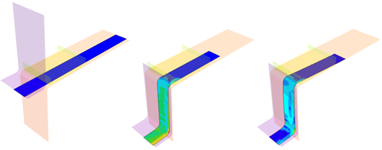
Fig 13: Deformed mesh of the sheet metal before and after the spring-back (multi-models mode).
The animations in Fig 14 include the results of the spring-back during simulation. There is an increasing number of stresses in the sheet metal from the start up to 960 ms, after which, the stresses begin to decrease as a result of the spring-back (stress relaxation).
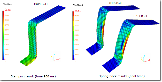
Fig 14: Stamping results on the sheet metal before and after spring-back.
Figure 15 shows the internal energy stored in the sheet metal during the stamping.
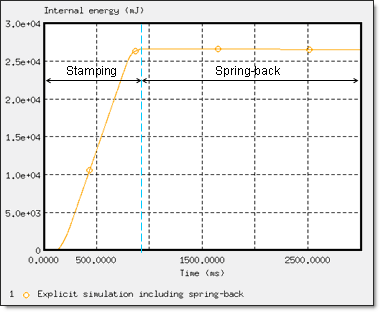
Fig 15: Internal energy in the sheet metal part (explicit spring-back simulation).
The dynamic relaxation used in the explicit spring-back computation enables to improve convergence towards quasi-static solution. The variation of the kinetics energy on the sheet metal in the explicit spring-back simulation is depicted in Fig 16 (from 960 ms up to 6000 ms):
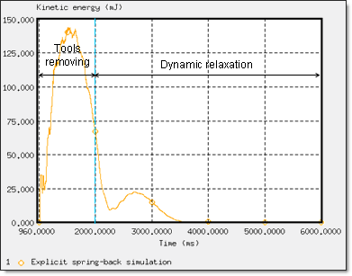
Fig 16: Convergence towards quasi-static equilibrium (explicit spring-back simulation).
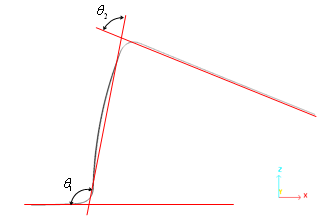
Comparison with experimental data on geometry after spring-back is shown in Table 1.
Table 1: Simulation results compared to experiment
|
|
|
Experiment |
105.7 |
77.7 |
Implicit |
100.8 |
78.6 |
Explicit |
106.1 |
78 |
The performance results are presented in Table 2.
Table 2: Implicit/explicit computation time.
|
Stamping CPU (cycles) |
Spring-back cycles |
Spring-back CPU (CPU per cycle) |
Total CPU |
|---|---|---|---|---|
Explicit |
1160 (92326) |
229379 (-) |
2698 (0.01) |
3858 |
Implicit |
- |
120 (354) |
1589 (13.2) |
2749 |
The implicit simulation for spring-back is performed from 960 ms to 1000 ms. Explicit spring-back simulation is performed until the kinetics energy on the sheet metal reaches a minimum value (quasi-static equilibrium). The final computation time is set to 6000 ms.
Explicit and implicit analysis' both obtain good results in this test, with implicit computation being 40% faster than the explicit computation. The implicit approach is; however, 1320 times more expensive per step than the explicit solver. The use of the implicit approach allows you to economize on the overall computation time.