Force: Contact

Model Element

Description

Force_Contact defines a 2-D or 3-D contact force between geometries on two rigid bodies. Each body is characterized by a set of one or more geometries which can be a 3D mesh or a 2D curve. Whenever any geometry on the first body penetrates any geometry on the second body, contact normal and frictional forces are generated. The normal force tends to repulse motion along the common normal at the contact point. The frictional force tends to oppose relative sliding velocity at the contact point. The contact force vanishes when the geometries no longer intersect.

Format

<Force_Contact

id = "integer"

[ label = "integer" ]

[ full_label = "string" ]

num_i_graphics = "integer"

i_graphics_id = "integer_list"

num_j_graphics = "integer"

j_graphics_id = "integer_list"

master_surface = { "I" | "J" | "I_and_J" | "AUTO" }

enable_sphere_to_mesh = {"TRUE" | "FALSE" }

contact_stability_2d = "real"

{

cnf_type = "POISSON"

penalty = "real"

restitution_coeff = "real"

normal_trans_vel = "real"

|

cnf_type = "IMPACT"

stiffness = "real"

exponent = "real"

damping = "real"

dmax = "real"

|

cnf_type = "VOLUME"

i_elastic_modulus = "real"

j_elastic_modulus = "real"

i_layer_depth = "real"

j_layer_depth = "real"

exponent = "real"

damping = "real"

|

cnf_type = "USERCNF"

cnf_param_string = "USER( [[par_1 [,...][,par_n]] )"

cnf_fnc_name = "string"

{ cnf_dll_name = "string"

|

script_name = "string"

interpreter = { "PYTHON" | "MATLAB" }

}

{

cff_type = "COULOMB_ON"

mu_static = "real"

mu_dynamic = "real"

stiction_trans_vel = "real"

friction_trans_vel = "real"

|

cff_type = "COULOMB_DYNAMICONLY"

mu_dynamic = "real"

friction_trans_vel = "real"

|

cff_type = "COULOMB_OFF"

|

cff_type = "USERCFF"

cff_param_string = "USER( [[par_1 [,...][,par_n]] )"

cff_fnc_name = "string"

{ cff_dll_name = "string"

|

script_name = "string"

interpreter = { "PYTHON" | "MATLAB" }

}

{

cpost_param_string = "USER( [[par_1 [,...][,par_n]] )"

cpost_fnc_name = "string"

{ cpost_dll_name = "string"

|

cpost_script_name = "string"

cpost_interpreter = "PYTHON"

}

Attributes

Element identification number (integer>0).

This is a number that is unique among all Force_Contact elements and uniquely identifies the element.

label

The name of the Force_Contact element. This argument is optional.

full_label

The full label of the Force_Contact element. This attribute is typically populated by MotionView as per the model hierarchy. This argument is optional.

num_i_graphics

Specifies the number of Post_Graphic elements on the first body that are to be considered in evaluating the contact force.

num_i_graphics > 0.

i_graphics_id

This is the list of the Post_Graphic element IDs on the first body to be considered for contact. The number of IDs in this list is specified by num_i_graphics.

Note: All the Post_Graphic entities must belong to the same body.

num_j_graphics

Specifies the number of Post_Graphic elements on the second body that are to be considered in evaluating the contact force.

num_j_graphics > 0

j_graphics_id

This is the list of the Post_Graphic element IDs on the second body to be considered for contact. The number of IDs in this list is specified by num_j_graphics.

Note: All the Post_Graphic entities must belong to the same body.

master_surface

Specifies which surface should be used as the master surface while calculating the penetration depth, point of contact, contact normal etc. You can choose from:

I: The geometry specified for the first body is the master.

J: The geometry specified for the second body is the master surface.

I_AND_J: Both the geometries for the first and second bodies are used as master surface alternatively and the result is summed up.

AUTO: Let MotionSolve decide which geometry to use as the master surface. This is the default option and is also the recommended option.

enable_sphere_to_mesh

Specifies whether MotionSolve should use an analytical description for sphere geometries defined in i_graphics_id or j_graphics_id. Choose from TRUE or FALSE.

The default is FALSE.

See Comment 1 for more details on usage.

contact_stability_2d

Specifies a stability value that is used when calculating the contact point and penetration depth in 2D curve contact.

The default value for this parameter is 0.1.

See Comment 10 for more details.

cnf_type

Specifies whether the POISSON, IMPACT, VOLUME or user defined (USERCNF) force model is to be used for calculating the contact normal force.

A contact force is computed as a function of the penetration between the intersecting geometries defined for the contact. In other words, as the geometries intersect, a repulsive force is generated which is based on the type of contact selected.

For more details on the different contact force models available in MotionSolve, please see Comment 2.

penalty (POISSON)

Specifies the stiffness parameter that is used to calculate the spring force. A large value for penalty permits only a small penetration between the two contacting geometries; a small value permits a larger penetration. Consider using a penalty value that is as small as possible, but still captures realistic deformation, to improve solver performance.

penalty > 0

restitution_coef (POISSON)

Defines the coefficient of restitution (COR) between the geometries in contact. This is used in the computation of the contact force. A value of zero specifies perfectly plastic contact meaning that the two bodies coalesce after contact. A value of one specifies perfectly elastic contact. No energy is lost in the collision and the relative velocity of separation equals the relative velocity of approach.

COR = (relative speed after collision)/(relative speed before collision)

1 > restitution_coef > 0

normal_trans_vel (POISSON)

Defines the velocity limit between the two bodies at which full damping is applied in the contact force. If unset by the user or set to 0, MotionSolve initializes it to 1. See Comment 4 for more details on this parameter’s use in the damping force.

stiffness (IMPACT)

The stiffness parameter of the contact; this is the same parameter as found for the IMPACT function. A large value for stiffness permits only a small penetration between the two contacting geometries; a small value permits a larger penetration. This parameter must be non-negative. Consider using a stiffness value that is as small as possible, but still captures accurate deformation, to improve solver performance.

stiffness > 0

exponent (IMPACT)

The exponent of the force deformation characteristic of the contact interface. For a stiffening spring characteristic, it must be greater than 1.0 and for a softening spring characteristic, it must be less than 1.0.

exponent > 0

damping (IMPACT)

The maximum damping coefficient. It must be non-negative.

damping > 0

dmax (IMPACT)

The penetration at which full damping is applied. It must be a positive number.

dmax > 0

i_elastic_modulus (VOLUME)

Specifies the elastic modulus for the geometries belonging to Body I for the Volume force model. The value of this elastic modulus can be derived from the Bulk and Shear Modulus of a material. See Comment 5 for more details on how this is calculated.

i_elastic_modulus > 0

j_elastic_modulus (VOLUME)

Specifies the elastic modulus for the geometries belonging to Body J for the Volume force model. The value of this elastic modulus can be derived from the Bulk and Shear Modulus of a material. See Comment 5 for more details on how this is calculated.

j_elastic_modulus > 0

i_layer_depth (VOLUME)

Specifies the size of the layer depth for the geometries belonging to body I. See Comment 5 for an explanation on how this parameter is used to calculate the contact stiffness.

i_layer_depth > 0

j_layer_depth (VOLUME)

Specifies the size of the layer depth for the geometries belonging to body I. See Comment 5 for an explanation on how this parameter is used to calculate the contact stiffness.

j_layer_depth > 0

exponent (VOLUME)

exponent > 0

damping (VOLUME)

The coefficient of damping used to calculate the damping force for the VOLUME force model

damping > 0

cnf_param_string (USERCNF)

Specify a list of parameters that are passed from the data file to the user written subroutine, CNFSUB.

cnf_dll_name (USERCNF)

Specifies the path and name of the shared library containing the contact force calculation subroutine. MotionSolve uses this information to load the user subroutine in the library at run time.

cnf_fnc_name (USERCNF)

Specifies an alternate name for the contact normal force subroutine, that is other than CNFSUB.

script_name (USERCNF, USERCFF)

Specifies the path and name of the user written script that contains the routine specified by cnf_fnc_name or cff_fnc_name.

interpreter (USERCNF, USERCFF)

Specifies the interpreted language that the user script is written in. Valid choices are MATLAB or PYTHON.

cff_type

Specifies the friction force model that will be used to compute the contact friction force. Choose from "COULOMB_ON", "COULOMB_OFF", "DYNAMIC_ONLY" or “USERCFF”.

cff_type = "COULOMB_ON" specifies that friction forces are to be calculated and applied at the contact location. MotionSolve uses the Coulomb model for friction force. See Comment 7 below.

cff_type = "COULOMB_OFF" specifies that frictional forces are not calculated or applied at the contact location. Friction is turned off.

cff_type = "COULOMB_DYNAMICONLY" specifies that only the dynamic friction is active. See Comment 7.

cff_type = "USERCFF" specifies that a user defined friction force model is to be used.

mu_static

Defines the coefficient of static friction when the friction is in the static regime.

MotionSolve uses a step function to transition between the static and dynamic friction regimes. See Comment 7 for more details.

mu_static > 0

mu_dynamic

Defines the coefficient of dynamic friction when the friction is in the dynamic regime.

MotionSolve uses a step function to transition between the static and dynamic friction regimes. See Comment 7 for more details. The coefficient of dynamic friction is smaller than or equal to the coefficient of static friction.

mu_static > = mu_dynamic > 0

stiction_trans_vel

The velocity at which the friction regime transitions to stiction. See Comment 7 for more details.

friction_trans_vel

The velocity at which the friction regime transitions to friction. See Comment 7 for more details.

|friction_trans_vel| >= |stiction_trans_vel|

cff_dll_name (USERCFF)

Specifies the path and name of the shared library containing the contact friction sub subroutine. MotionSolve uses this information to load the user subroutine in the library at run time.

cff_fnc_name (USERCFF)

Specifies an alternate name for the contact normal force subroutine i.e. other than CFFSUB.

cff_param_string (USERCFF)

Specify a list of parameters that are passed from the data file to the user written subroutine, CFFSUB.

cpost_dll_name

Specifies the path and name of the shared library containing the contact post sub subroutine. MotionSolve uses this information to load the user subroutine in the library at run time.

cpost_fnc_name

Specifies an alternate name for the contact post subroutine i.e. other than CONTACTPOST.

cpost_param_string

Specify a list of parameters that are passed from the data file to the user written subroutine, CONTACTPOST.

cpost_interpreter

Specifies the interpreted language that the user script is written in. Currently, only Python is supported as an interpreter for the CONTACTPOST subroutine.

cpost_script_name

Specifies the path and name of the user written script that contains the routine specified by cpost_fnc_name.

Comments

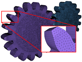
1.	Computing a contact force between two bodies requires a geometrical representation of the two bodies. MotionSolve allows you to define contact between rigid bodies in two ways:

Using a 3D representation: This geometrical representation of the body is termed a graphic for that body. MotionSolve relies on a collision engine to detect intersection or penetration between two graphics. To do this, the collision engine requires the graphics to be meshed using triangular elements. A meshed graphic is a set of interconnected triangular elements. This is illustrated in the figure below:

fc_model_comment1_fig1

Geometrical representation of two gear bodies

fc_model_comment1_fig2

Meshed representation of the same gear bodies

MotionSolve prescribes certain conditions for the meshed representation of a body’s graphic(s). These conditions must be met to generate realistic contact forces. These are:

a)	Only triangular shell elements are allowed in the meshed representation. Quadrilateral or other shell elements are not permitted.

b)	The mesh must be a surface mesh i.e. a mesh comprised of 2-D triangular shell elements with no thickness. Solid meshes that make use of tetrahedral, hexahedral or other element types are not required.

c)	The mesh must enclose a volume i.e. it must be closed. In other words, there must not be any free edges or cracks in the mesh. For example, a flat surface with zero volume is not allowed.

d)	T-connections are not allowed in the mesh – this means that an edge of a triangular element must be shared by no more than two elements.

e)	The surface normal for a meshed representation of a body’s graphic(s) must point outward from the surface that can come into contact. The direction of these normals may be flipped in MotionView by toggling the “Material Inside” check box in the MotionView contact panel.

For more information on these rules, please refer to the help topic Best Modeling Practices for 3D Contacts in the MotionSolve User's Guide.

Graphics for rigid bodies may be defined in many ways:

•

For spherical geometries, MotionSolve can use an analytical description of the geometry (based on a radius and a location for the center of the sphere) while computing the contact point, contact normal and other quantities. This approach is followed whenever MotionSolve detects a primitive sphere geometry (of type = “SPHERE” in Post_Graphic) for Body I or Body J or both. There are two advantages of using an analytical description for a spherical body:

o	Since there is no surface mesh, there are no errors due to the approximation of the surface by a triangulated mesh. This means the contact forces are more accurate

o	The solution time is typically much smaller for contact involving a sphere and a generalized 3D mesh

To force MotionSolve to use a meshed representation of the sphere geometry, you can specify enable_sphere_to_mesh to be FALSE. This way, MotionSolve will mesh the primitive sphere geometry and use the meshed representation of the sphere to compute the contact related quantities.

•	For simple shapes, you may use built in primitive graphics provided by MotionSolve such as Sphere, Frustum, Box etc. For these primitive shapes, MotionSolve meshes the surface internally using the attribute refinement_level to determine the density of the mesh

More complicated shapes can be defined in a CAD package and imported to MotionSolve using the Import CAD Tool in MotionView. Please see Import CAD or FE for more information on how CAD geometry can be meshed using this tool. Alternatively, you may also use HyperMesh to mesh your CAD graphics.

Using a 2D representation: MotionSolve also supports contact between two curves that represent two rigid bodies. 2D curve graphics can be specified by referencing a Post_Graphic of type = ”CURVE”. Using 2D curve-based contact can be advantageous over 3D mesh-based contact when:

1.	It is known a priori that the contact occurs only along the curves that are defined. Further, contact is expected to occur within the plane in which the two curves are defined. In other words, there are no out-of-plane contact forces that are expected.

2.	The curves between which the contact is to be calculated are smooth and represent the curvature of the 3D geometry well.

There may be several advantages of simulating rigid body contact using 2D curves over 3D tessellated geometry:

1.	More accurate results: Results are more accurate since there is less error due to discretization. Discretization of 3D geometry into triangles occurs over three dimensions as opposed to two in curves.

Easily improve accuracy: Result accuracy can be improved rapidly by introducing more points in the curve within MotionView. Improving the accuracy of results when using 3D contact requires you to re-import the graphic and re-mesh, or go outside the MotionView environment into a CAD tool to re-mesh. Re-meshing a 3D geometry takes more time than refining a 2D curve.

3.	Faster simulation times: For geometries where contact occurs over a curve, using a curve-curve contact is much faster than using a 3D tessellated geometry since the solver has to work harder to determine contact for a 3D tessellated geometry which increases the overall simulation time

As with 3D mesh-based contact, certain restrictions apply:

1.	Curves have to be flat and defined in the x-y plane relative to the reference marker specified in Post: Graphic.

2.	CURSUB routines are currently not supported.

3.	All i_graphic_id's and all j_graphic_id’s have to point to curve graphics, which are defined in the same plane.

4.	The z-direction of each graphic reference marker has to point in the same direction.

5.	You must ensure that the graphics will remain in one plane during simulation. The easiest way to achieve this is by adding an inplane joint to the model.

Note: 2D curve contact uses a smooth representation of the specified curves which is independent of the nseg specified in Post: Graphic.

2.	Three pre-defined contact force models are available for computing the normal force: POISSON, IMPACT and VOLUME. If none of these is suitable, you may write your own force model as a subroutine or script and use that to compute the normal contact force.

The normal force computed in the POISSON, IMPACT and VOLUME methods consists of two components: an elastic spring force and a dissipative damping force. Each method has its own way of computing these forces, described in the subsequent comments.

3.	In the IMPACT model, the contact normal force is modeled with the IMPACT function. The penetration depth and rate are computed by the collision detection algorithm and fed into the IMPACT function. See the IMPACT function for more details.

	Stiffness
	Contact penetration depth
	Exponent for the force deformation characteristic
	Penetration depth at which full damping is applied
	Damping coefficient

4.	In the POISSON model, the elastic spring force component of the normal force is modeled using the Hertz contact theory, while the damping force uses the coefficient of restitution and a user defined velocity limit as part of the calculation. The equations that define this force are listed below.

	Penalty parameter (stiffness).
	Contact penetration depth.
	The coefficient of restitution. This is equal to 0 for a perfectly plastic collision and 1 for a perfectly elastic collision.
	Normal velocity at which full damping is applied.

Note:For a coefficient of restitution = 0, when the two bodies are colliding head to head, and dz/dt > vnorm_trans, then the damping force is equal to the spring force, and the total contact normal force is zero.

In this model, the energy loss is modeled with a coefficient of restitution. Table 1 lists the coefficient of restitution for some materials. Contact is assumed to be between like materials, for example, Brass-Brass, Steel-Steel, and so on.

Material	Coefficient of Restitution
Brass	0.30
Bronze	0.52
Copper	0.22
Cork	0.60
Elm	0.48
Glass	0.96
Iron	0.67
Ivory	0.78
Lead	0.16
Maple	0.65
Rubber	0.75
Steel	0.90

Table 1: Coefficient of restitution for common materials

5.	In the VOLUME model, the elastic spring force component of the normal force is modeled similar to the IMPACT model, while the damping force uses a damping coefficient to compute the damping force. The equations that define this force are listed below.

where

	Contact stiffness.
	Contact penetration depth.
	Exponent for the force deformation characteristic.
	Damping coefficient.
	Area of contact.

The VOLUME model assumes that both the colliding bodies are surrounded by a layer of springs whose stiffness is determined by the material’s elastic modulus properties and the depth of this layer. The individual stiffness for each body (I and J) is calculated as

where,

	Stiffness parameter for I and J bodies, respectively.
	Elastic Modulus for I and J bodies, respectively.
	Layer depth for I and J bodies, respectively.

The equivalent contact stiffness is calculated assuming that the springs for body I and J are in series:

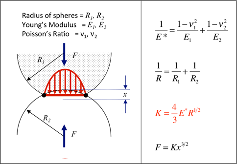
Note: The equivalent stiffness calculated above has units of Force per cubic length. The VOLUME force method utilizes the contact area and penetration depth to retrieve the contact force in Newton (or the model unit for force).

The elastic modulus M (sometimes also called P-wave modulus) for both the bodies in contact is calculated using the Bulk and Shear Modulus of their respective materials. These can be specified in the Contact panel in MotionView. The elastic modulus is calculated as

where,

	Elastic or P-wave modulus.
	Bulk Modulus.
	Shear Modulus.

The Bulk and Shear Modulus for homogenous, isotropic materials can be calculated from the Young’s Modulus and Poisson ratio as

where,

	Young’s modulus
	Poisson ratio

Both the elastic modulus and layer depth determine the value of the equivalent contact stiffness. Since for a given material, the elastic modulus is typically a constant value, you may change the layer depth to obtain an appropriate penetration in your model. For example, assume that two steel bodies are in contact. For steel (G = 160GPa, K = 79GPa), M = 292.33GPa. If you specify the layer depth to be 100mm, the contact stiffness is ~1.461E+03 N/mm3. If you reduce this layer depth by a factor of 10, i.e. 10mm, the contact stiffness goes up by a factor of 10 i.e. ~1.461E+04 N/mm3.

The VOLUME force model thus lets you derive the contact stiffness from physical material properties of the colliding bodies.

6.	A good first estimate for the stiffness parameters (for both POISSON and IMPACT models) can be obtained by making use of the classical Hertzian contact theory for non-adhesive contact. The general case for contact between two spherical bodies of radius R1 and R2 is illustrated in the image below.

fc_model_comment6_fig1

Figure 2: Hertzian contact stiffness for two spherical objects

Hertz theory is developed using static load cases. The stiffness is a function of the material properties of the two bodies in contact as well as the geometry at the contact patch. The stiffness coefficient is shown in red.

Assume that two steel balls are in contact. The radii of the steel balls are 30mm; the Young’s modulus for steel is 200 GPa; Poisson’s ratio for steel is 0.3. Using the formula shown above, the stiffness coefficient for contact is: K = 1.7945E+10 N/m = 1.7945E+07 N/mm

This should be considered a starting point for the penalty or stiffness value. You may need to tune this parameter, as high values of stiffness can degrade the performance of the solver. However, you may find that you are able to allow a smaller penalty, and thus more penetration, and still capture the overall system behavior.

7.	Two friction models are supported in MotionSolve

•	Coulomb model of friction which calculates the friction force as the normal force multiplied by the coefficient of friction. This coefficient is calculated as a function of the slip velocity that is explained below

•	A user defined friction force model that can be implemented as a subroutine or a script

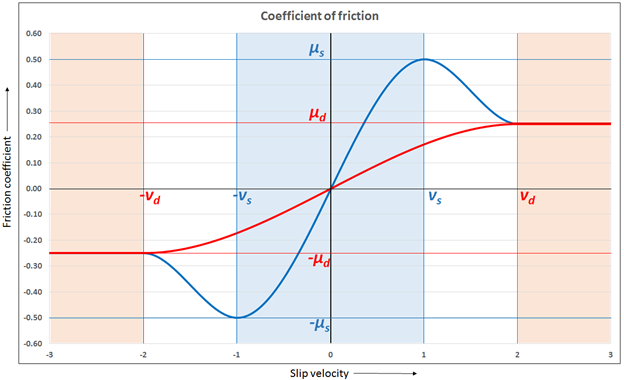
For the first approach, the friction force at the contact patch is computed in the same manner for POISSON, IMPACT and VOLUME force models. The Coulomb friction law is used which models the friction force as a coefficient of friction multiplied by the normal force. The coefficient of friction is modeled as a function of the slip velocity. The frictional force is modeled as a viscous force according to the following equations:

where,

is the current slip speed at the point of contact

is the stiction transition slip speed at which the full value of is used for the coefficient of friction

is the dynamic friction slip speed at which the full value of is used for the coefficient of friction

is the coefficient of static friction

is the coefficient of dynamic friction

Figure 3 illustrates the functional relation between coefficient of friction and slip velocity

The red curve depicts the full friction model covering all three regimes: static, transition to sliding friction, and sliding friction. This is the friction model applied when you select cff_type = "COULOMB_ON".

The blue curve depicts the friction model covering only the sliding friction regime. This is the friction model applied when you select cff_type = "DYNAMICS_ONLY".

FC_ComFig2

Figure 3: Coefficient of friction as a function of slip velocity

The blue curve depicts the full friction model covering all three regimes. These are:

•	The static regime shown in light blue

•	The transition from static to dynamic friction show in white

•	The dynamic friction regime shown in light pink.

This is the friction model applied when you select cff_type = "COULOMB_ON".

The red curve depicts the friction model covering only the sliding friction regime. This is the friction model applied when you select cff_type = "DYNAMICS_ONLY".

μ is the friction coefficient that is to be applied. The friction force opposes the direction of the slip velocity. The table below lists the coefficient of friction for some common material pairs. The friction values are extremely sensitive to surface coatings, so both dry and greasy values are specified.

Material 1	Material 2	Coefficient Of Friction
		Dry		Greasy
		Static	Sliding	Static	Sliding
Aluminum	Aluminum	1.05-1.35	1.4	0.3
Aluminum	Mild Steel	0.61	0.47
Brake Material	Cast Iron	0.4
Brake Material	Cast Iron (Wet)	0.2
Brass	Cast Iron		0.3
Brick	Wood	0.6
Bronze	Cast Iron		0.22
Bronze	Steel			0.16
Cadmium	Cadmium	0.5		0.05
Cadmium	Mild Steel		0.46
Cast Iron	Cast Iron	1.1	0.15		0.07
Cast Iron	Oak		0.49		0.075
Chromium	Chromium	0.41		0.34
Copper	Cast Iron	1.05	0.29
Copper	Copper	1		0.08
Copper	Mild Steel	0.53	0.36		0.18
Copper	Steel		0.8
Copper	Steel (304 stainless)	0.23	0.21
Copper-Lead Alloy	Steel	0.22		-
Diamond	Diamond	0.1		0.05 - 0.1
Diamond	Metal	0.1 -0.15		0.1
Glass	Glass	0.9 - 1.0	0.4	0.1 - 0.6	0.09-0.12
Glass	Metal	0.5 - 0.7		0.2 - 0.3
Glass	Nickel	0.78	0.56
Graphite	Graphite	0.1		0.1
Graphite	Steel	0.1		0.1
Graphite (In vacuum)	Graphite (In vacuum)	0.5 - 0.8
Hard Carbon	Hard Carbon	0.16		0.12 - 0.14
Hard Carbon	Steel	0.14		0.11 - 0.14
Iron	Iron	1		0.15 - 0.2
Lead	Cast Iron		0.43
Lead	Steel		1.4
Leather	Wood	0.3 - 0.4
Leather	Metal(Clean)	0.6		0.2
Leather	Metal(Wet)	0.4
Leather	Oak (Parallel grain)	0.61	0.52
Magnesium	Magnesium	0.6		0.08
Nickel	Nickel	0.7-1.1	0.53	0.28	0.12
Nickel	Mild Steel		0.64;		0.178
Nylon	Nylon	0.15 - 0.25
Oak	Oak (parallel grain)	0.62	0.48
Oak	Oak (cross grain)	0.54	0.32		0.072
Platinum	Platinum	1.2		0.25
Plexiglas	Plexiglas	0.8		0.8
Plexiglas	Steel	0.4 - 0.5		0.4 - 0.5
Polystyrene	Polystyrene	0.5		0.5
Polystyrene	Steel	0.3-0.35		0.3-0.35
Polythene	Steel	0.2		0.2
Rubber	Asphalt (Dry)		0.5-0.8
Rubber	Asphalt (Wet)		0.25-0.0.75
Rubber	Concrete (Dry)		0.6-0.85
Rubber	Concrete (Wet)		0.45-0.75
Sapphire	Sapphire	0.2		0.2
Silver	Silver	1.4		0.55
Sintered Bronze	Steel	-		0.13
Solids	Rubber	1.0 - 4.0		--
Steel	Aluminum Bros	0.45
Steel	Brass	0.35		0.19
Steel(Mild)	Brass	0.51	0.44
Steel (Mild)	Cast Iron		0.23	0.183	0.133
Steel	Cast Iron	0.4		0.21
Steel	Copper Lead Alloy	0.22		0.16	0.145
Steel (Hard)	Graphite	0.21		0.09
Steel	Graphite	0.1		0.1
Steel (Mild)	Lead	0.95	0.95	0.5	0.3
Steel (Mild)	Phos. Bros		0.34		0.173
Steel	Phos Bros	0.35
Steel(Hard)	Polythened	0.2		0.2
Steel(Hard)	Polystyrene	0.3-0.35		0.3-0.35
Steel (Mild)	Steel (Mild)	0.74	0.57		0.09-0.19
Steel (Mild)	Steel (Mild)	-	0.62
Steel(Hard)	Steel (Hard)	0.78	0.42	0.05 -0.11	0.029-.12
Steel	Zinc (Plated on steel)	0.5	0.45	-	-
Teflon	Steel	0.04		0.04	0.04
Teflon	Teflon	0.04		0.04	0.04
Tin	Cast Iron		0.32
Titanium Alloy Ti-6Al-4V(Grade 5)	Aluminum Alloy 6061-T6	0.41	0.38
Titanium Alloy Ti-6Al-4V(Grade 5)	Titanium Alloy Ti-6Al-4V(Grade 5)	0.36	0.3
Titanium Alloy Ti-6Al-4V(Grade 5)	Bronze	0.36	0.27
Tungsten Carbide	Tungsten Carbide	0.2-0.25		0.12
Tungsten Carbide	Steel	0.4 - 0.6		0.08 - 0.2
Tungsten Carbide	Copper	0.35
Tungsten Carbide	Iron	0.8
Wood	Wood(clean)	0.25 - 0.5
Wood	Wood (Wet)	0.2
Wood	Metals(Clean)	0.2-0.6
Wood	Metals (Wet)	0.2
Wood	Brick	0.6
Wood	Concrete	0.62
Zinc	Zinc	0.6		0.04
Zinc	Cast Iron	0.85	0.21

9.	The current implementation of the contact force modeling in MotionSolve has some limitations.

•	It is only supported for rigid body and point mass objects. Contact between flexible bodies is not supported.

•	Stiction or stick-slip phenomena are not supported at this time.

10.

For 2D curve contact, the contact point is determined as the point of maximum penetration in the direction of the contact normal. For configurations that yield deep penetrations between curves, it is possible that this point is not uniquely defined. In such a situation, the parameter contact_stability_2d can be added. The parameter adds a virtual spring in the contact point calculation that pulls the point of contact in the direction of the center of mass of the overlapping area. A larger value yields a stronger spring and thus a larger stability. The penetration depth is calculated based on the distance in the normal direction of the contact point found in this way.

If the contact_stability_2d is set to zero, contact point calculation will be skipped and the center of mass of the overlapping area will be used instead. In this case, penetration depth will be calculated based on the overlapping area. This value usually slightly underestimates the true penetration depth.

Debugging Tips

•	Confirm that models run without contact before adding them.

•	Start modeling with contact friction off, and add it later after getting the normal force running.

•	Some experimentation is usually required for tuning the contact parameters to get realistic and stable results.

•

Small values for stiction_trans_vel and friction_trans_vel cause the integrator to take too small of steps when the coefficient of friction is large. Increase the value for stiction_trans_vel if you are experiencing integration difficulties. In our experience, this does not change the results significantly.

•

Large values for the penalty or stiffness decreases the penetration allowed between geometries; however they also tend to decrease the integrator step size. Consider allowing as much penetration of the geometries as will still capture the behavior of the system that you’re interested in measuring. This will be model-dependent. The contact force computation will be much smoother in general if a moderate amount of penetration (due to a lower stiffness/penalty) is allowed. Ask yourself, “Will 0.1 mm of penetration change the behavior of my system? Will 1 mm?”

•	In general, a finer mesh at the contact surface may help obtain more accurate results. However, a fine mesh also increases the computational effort of the collision-detection algorithm, which may slow down the simulation.

•	Check the normals of the geometries to make sure that they have been defined properly for the contact. In the Tria mesh geometry, the normal is defined by a right-hand rule of the mesh nodes. For example, you can view the normals using the check normals tool in the Contact panel in MotionView.

•	If the contacts are not detected or pass through each other during the simulation, try one of the following: decreasing the integrator step size (for example, h_max), decreasing the error tolerance, increasing the penalty/stiffness (if too soft), or checking the element normals.

Alternatively, you can turn on the “zero crossing” action for the contact sensor in the Contact panel in MotionView. By doing this, MotionSolve will attempt to determine the moment of first contact more accurately which may alleviate this problem. For more information on this sensor, please refer to the documentation for Sensor_Event.

•

If the integrator fails, use DebugOutput to determine if the contact is causing problems. If it is, then try one of the following: decreasing the contact penalty/stiffness and/or damping (if too large), decreasing h_max, increasing the integrator error tolerance, adding damping to other stiff entities in the model, or tuning the contact friction parameter as described previously.

Limitations

The current implementation of Force_Contact has some limitations.

•	It is only supported for rigid body and point mass objects. Flexible bodies are not supported.

•	Contact between 2-D geometries, such as curves, arcs, and circles, is not supported at this time.

Example

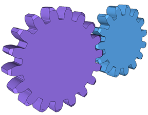
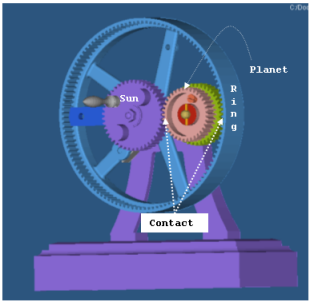
The image below demonstrates an epicyclic gear train that is used in a child’s toy. When the child cranks the sun gear, the other gears rotate.

The gear train consists of two contacts: one between the Sun gear and the Planet gear, and a second between the Planet gear and the Ring gear. The gears are made out of copper, and some oil is used to lubricate the system.

FC_ExFig1

Figure 4: An epicyclic gear train used in a child’s toy

The Force_Contact statements for this example are shown below. The system is modeled in SI units.

The first contact is between the Sun gear and the Planet gear.

<Force_Contact

id = "1"

num_i_graphics = "1"

i_graphics_id = "82"

num_j_graphics = "1"

j_graphics_id = "92"

cnf_type = "POISSON

penalty = "1E6"

restitution_coef = "0.52"

cff_type = "COULOMB_ON"

mu_static = "0.08"

mu_dynamic = "0.05"

stiction_trans_vel = "0.005"

friction_trans_vel = "0.01"

The second contact, shown below, is between the Planet and the Ring gears.

<Force_Contact

id = "2"

num_i_graphics = "1"

i_graphics_id = "93"

num_j_graphics = "1"

j_graphics_id = "73"

cnf_type = "POISSON"

penalty = "1E6"

restitution_coef = "0.52"

cff_type = "COULOMB_ON"

mu_static = "0.08"

mu_dynamic = "0.06"

stiction_trans_vel = "0.005"

friction_trans_vel = "0.0l"

For a more detailed example, see the tutorial MV-1010: Contact Simulation using MotionSolve.

Model Element
Description
CONTACT defines a 3-D contact force between geometries on two rigid bodies. Each body is characterized by a set of one or more geometries. Whenever any geometry on the first body penetrates any geometry on the second body, a contact normal and frictional force are generated. The normal force tends to repulse motion along the common normal at the contact point. The frictional force tends to oppose relative sliding velocity at the contact point. The contact force vanishes when the geometries no longer intersect.
Declaration
def CONTACT(id, LABEL="", IGEOM=[], JGEOM=[], TYPE="", STIFFNESS=0.0, EXPONENT=0.0, DAMPING=0.0, DMAX=0.0, PENALTY=0.0, RESTITUTION_COEFFICIENT=0.0, COULOMB_FRICTION="Off", MU_STATIC=0.0, MU_DYNAMIC=0.0, STICTION_TRANSITION_VELOCITY=0.0, FRICTION_TRANSITION_VELOCITY=0.0, I_ELASTIC_MODULUS=0.0, I_LAYER_DEPTH=0.0, J_ELASTIC_MODULUS=0.0, J_LAYER_DEPTH=0.0, MASTER_SURFACE="", COLLISION_ENGINE="", NORMAL_ROUTINE="", FRICTION_ROUTINE="", NORMAL_FUNCTION="", FRICTION_FUNCTION=""):
Attributes
id	This is a number that is unique among all CONTACT elements and uniquely identifies the element.
LABEL	The name of the CONTACT element. This argument is optional.
IGEOM	This is a list of the GRAPHICS element IDs on the first body to be considered for contact. Note All the GRAPHICS entities must belong to the same body.
JGEOM	This is a list of the GRAPHICS element IDs on the second body to be considered for contact. Note All the GRAPHICS entities must belong to the same body.
TYPE	Specifies whether the POISSON, IMPACT, VOLUME, or USER defined force model is to be used for calculating the contact normal force. A contact force is computed as a function of the penetration between the intersecting geometries defined for the contact. In other words, as the geometries intersect, a repulsive force is generated which is based on the type of contact selected. If TYPE is not specified or equal to zero, the IMPACT contact force model will be used.
STIFFNESS	The stiffness parameter of the contact; this is the same parameter as found for the IMPACT function. A large value for stiffness permits only a small penetration between the two contacting geometries; a small value permits a larger penetration. This parameter must be non-negative. Consider using a stiffness value that is as small as possible, but still captures accurate deformation, to improve solver performance.
EXPONENT	The exponent of the force deformation characteristic of the contact interface. For a stiffening spring characteristic, it must be greater than 1.0 and for a softening spring characteristic, it must be less than 1.0.
DAMPING	The maximum damping coefficient. It must be non-negative.
DMAX	The penetration at which full damping is applied. It must be a positive number.
PENALTY	Specifies the stiffness parameter that is used to calculate the spring force. A large value for PENALTY permits only a small penetration between the two contacting geometries; a small value permits a larger penetration. Consider using a penalty value that is as small as possible, but still captures realistic deformation, to improve solver performance.
RESTITUTION_COEFFICIENT	Defines the coefficient of restitution (COR) between the geometries in contact. This is used in the computation of the contact force. A value of zero specifies perfectly plastic contact meaning that the two bodies coalesce after contact. A value of one specifies perfectly elastic contact. No energy is lost in the collision and the relative velocity of separation equals the relative velocity of approach. COR = (relative speed after collision)/(relative speed before collision)
COULOMB_FRICTION	Specifies the friction force model that will be used to compute the contact friction force. Choose from "ON", "OFF", "DYNAMICS_ONLY". "ON" specifies that friction forces are to be calculated and applied at the contact location. MotionSolve uses the Coulomb model for friction force. "OFF" specifies that frictional forces are not calculated or applied at the contact location. Friction is turned off. "DYNAMICONLY" specifies that only the dynamic friction is active. If FRICTION_FUNCTION/ FRICTION_ROUTINE is specified it will be used instead of the previous selected method.
MU_STATIC	Defines the coefficient of static friction when the friction is in the static regime. MotionSolve uses a step function to transition between the static and dynamic friction regimes.
MU_DYNAMIC	Defines the coefficient of dynamic friction when the friction is in the dynamic regime. MotionSolve uses a step function to transition between the static and dynamic friction regimes. The coefficient of dynamic friction is smaller than or equal to the coefficient of static friction.
STICTION_TRANSITION_VELOCITY	Defines the slip velocity at which the static coefficient of friction, MU_STATIC, is applied.
FRICTION_TRANSITION_VELOCITY	Defines the slip velocity at which the dynamic coefficient of friction, MU_DYNAMIC, is applied.
I_ELASTIC_MODULUS	Specifies the elastic modulus for the geometries belonging to Body I for the Volume force model. The value of this elastic modulus can be derived from the Bulk and Shear Modulus of a material.
I_LAYER_DEPTH	Specifies the size of the layer depth for the geometries belonging to body I.
J_ELASTIC_MODULUS	Specifies the elastic modulus for the geometries belonging to Body J for the Volume force model. The value of this elastic modulus can be derived from the Bulk and Shear Modulus of a material.
J_LAYER_DEPTH	Specifies the size of the layer depth for the geometries belonging to body I.
MASTER_SURFACE	Specifies which surface should be used as the master surface while calculating the penetration depth, point of contact, contact normal, and so on. You can choose from: “I”: The geometry specified for the first body is the master. “J”: The geometry specified for the second body is the master surface. “IANDJ”: Both the geometries for the first and second bodies are used as master surface alternatively and the result is averaged. “AUTO”: Let MotionSolve decide which geometry to use as the master surface. This is the default option and is also the recommended option.
COLLISION_ENGINE	Specifies which collision engine should be used for contact detection. Choose from "AUTO", "OPCODE" or "PCM".
NORMAL_ROUTINE	Specifies the path and name of the shared library containing the contact force calculation subroutine. MotionSolve uses this information to load the user subroutine in the library at run time.
FRICTION_ROUTINE	Specifies the path and name of the shared library containing the friction force calculation subroutine. MotionSolve uses this information to load the user subroutine in the library at run time
NORMAL_FUNCTION	The list of parameters that are passed from the data file to the user defined subroutine. The user defined subroutine CNFSUB is used.
FRICTION_FUNCTION	The list of parameters that are passed from the data file to the user defined subroutine. The user defined subroutine CFFSUB is used.
Comments See Force_Contact
Example The example below shows a sample contact definition. CONTACT(1, IGEOM=[82], JGEOM=[92], TYPE="POISSON", COULOMB_FRICTION="ON", PENALTY =1000000, RESTITUTION_COEFFICIENT =0.52, AUGMENTED_LAGRANGIAN_FORMULATION=True, MU_STATIC =0.08, MU_DYNAMIC =0.05, STICTION_TRANSITION_VELOCITY = 0.005, FRICTION_TRANSITION_VELOCITY =0.01)