Summary
Four cantilever beams are analyzed. The objective is to evaluate the response of the beams under (i) linear static analysis (small displacements) and (ii) geometric nonlinear analysis (large displacements) with and without the application of follower forces.
Considering the example is a static problem, the nonlinear implicit solver is used.
Title
Follower Force
|
|
Number
41.1
|
Brief Description
Cantilever beams.
|
Keywords
| • | Nonlinear large displacement analysis (NLGEOM) |
| • | Termination time (TTERM) |
|
OptiStruct Options
| • | Parameters for Geometric Nonlinear Implicit Static Analysis Control (NLPARMX) |
| • | Boundary conditions (SPC) |
| • | Default shell element parameters (XSHLPRM) |
| • | Fixed coordinate system (CORD2R) |
| • | Moving coordinate system (CORD3R) |
|
Input File
Follower force: <install_directory>/demos/hwsolvers/optistruct/follow_force.fem
|
Technical / Theoretical Level
Beginner
|
Overview
Aim of the Problem
Follower forces imply that the direction of the load is assumed to rotate with the rotation at the node (where the load is applied). The purpose of this example is to compare the deformation characteristics of several cantilever beams – with and without the application of follower forces in a geometrically nonlinear implicit analysis (NLGEOM) and that in a geometrically linear static analysis.
Physical Problem Description
The four beams are all identical with a length of 100mm, width of 10mm and thickness of 1mm.
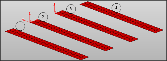
Fig 1: Geometry of the beams.
Small displacement (linear static) analysis is performed on beam 1. Large displacement (NLGEOM) analysis is performed on beams 2, 3 and 4, as shown in Figure 1.
The material used is elastic with the following properties:
| • | Young’s modulus: 2.1e+5 MPa |
Analysis, Assumptions and Modeling Description
Modeling Methodology
The mesh is a regular shell mesh with average element size of 5mm.
The beams have been modeled using first order reduced integrated shell elements as specified in the default definition of shell element properties (XSHLPRM):
PSHELL 1 11.0 1 1 0.0
XSHLPRM 24 2 VAR NEWT 5
The loads and boundary conditions applied in the model are shown in Figure 2.
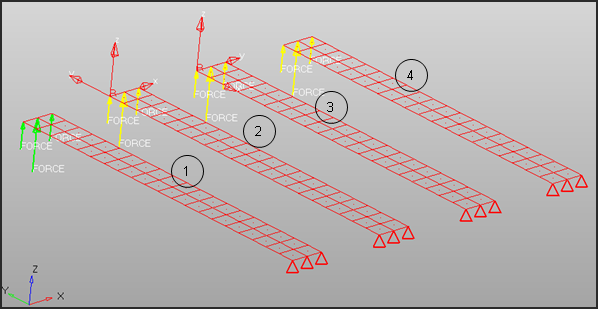
Fig 2: Loads and Boundary conditions
The cantilever beams are constrained at one end and all dof and forces are applied at the other end (15N are applied at the the two outer nodes as 30N is applied at the center node).
SPC 6 1 1234560.0
………………
For NLGEOM analysis, the loading is defined using NLOAD1 card:
TABLED1 8 LINEAR LINEAR
+ 0.0 0.0 1.0 1.0ENDT
NLOAD1 7 4 8
Force Type – Follower or Non-follower
For beams 1 and 4, the loading is defined in default global coordinate system, which is a fixed coordinate system, signifying the definition of non-follower force on both the beams. Static analysis is performed on beam 1, while geometric nonlinear analysis is performed on beam 4.
For beam 2, loading is defined with a fixed coordinate system (CORD2R) signifying the definition of non-follower force on this beam as well. Geometric nonlinear analysis is performed on beam 2.
CORD2R 1 30.0 100.0 0.0 30.0 100.0 100.0
+ 130.0 100.0 0.0
FORCE 4 88 11.0 0.0 0.0 15.0
FORCE 4 89 11.0 0.0 0.0 30.0
FORCE 4 90 11.0 0.0 0.0 15.0
For beam 3, loading is defined with a moving coordinate system (CORD3R) signifying the follower force on beam 3. Geometric nonlinear analysis is performed on beam 3.
CORD3R 3 151 150 178
FORCE 4 151 31.0 0.0 0.0 15.0
FORCE 4 152 31.0 0.0 0.0 30.0
FORCE 4 153 31.0 0.0 0.0 15.0
OptiStruct Options Used
As mentioned before, small displacement linear static analyses (for beam 1), as well as large displacement nonlinear implicit analyses (for beams 2, 3 and 4) have been performed in this example. The nonlinear analysis is performed using the arc-length displacement strategy. The time step is determined by a displacement norm control.
The nonlinear implicit parameters used are:
Implicit type:
|
Static nonlinear
|
Nonlinear solver:
|
Modified Newton method
|
Termination criteria:
|
Relative residual in force and energy
|
Tolerance:
|
0.01
|
Update of stiffness matrix:
|
5 iterations maximum
|
Time step control method:
|
Arc-length
|
Initial time step:
|
0.5
|
Minimum time step:
|
1e-5
|
Maximum time step:
|
1.5
|
Line search method:
|
ENERGY
|
Desired convergence iteration number:
|
6
|
Maximum convergence iteration number:
|
20
|
Decreasing time step factor:
|
0.67
|
Maximum increasing time step scale factor:
|
1.1
|
Arc-length:
|
Automatic computation
|
Spring-back option:
|
No.
|
A solver method is required to resolve Ax=b in each iteration of a nonlinear cycle. The linear implicit options used are:
Linear solver:
|
Direct (BCS)
|
Precondition methods:
|
Factored approximate Inverse
|
Maximum iterations number:
|
System dimension (NDOF)
|
Stop criteria:
|
Relative residual of preconditioned matrix
|
Tolerance for stop criteria:
|
Machine precision
|
The input nonlinear implicit options set in the FEM file are defined by NLPARMX:
NLPARM 1 2
+
NLPARMX 1 0.0 0.1 0.01 -1 40
Refer to the OptiStruct manual for more details about implicit options.
The nonlinear large deformation analysis has to be defined through a subcase. An NLPARM statement, as well as ANALYSIS=NLGEOM has to be present in the subcase. The termination time of 1.0s is defined through the TTERM entry. The first subcase is linear static and the second subcase is geometric nonlinear.
$HMNAME LOADSTEP 1"linstatic" 1
$
SUBCASE 1
SPC = 6
LOAD = 2
$
$HMNAME LOADSTEP 2"nlgeom" 15
$
SUBCASE 2
ANALYSIS NLGEOM
SPC = 6
NLPARM = 1
NLOAD = 7
TTERM = 1.0
Simulation Results and Conclusions
Animations
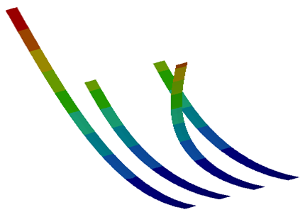
The displacement contour on the beams is shown in Figure 3. As expected, beam 1 for which static analysis has been performed, shows the largest deformation. Beam 2 (for which loading has been defined in a fixed coordinate system) and beam 4 (for which loading has been defined in the default global coordinate system) show the exact same deformations. Beam 3 for which NLGEOM analysis has been performed with follower forces, shows higher deformations than beams 2 and 4, and the end where load is applied bulges out into a spherical shape.
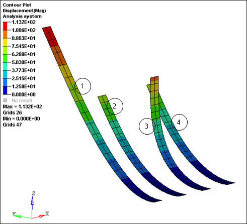
Fig 3: Displacement contour of the four cantilever beams
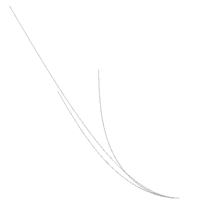
Figure 4 shows the differences in deformation characteristics with and without the application of follower forces for geometrically linear and geometrically nonlinear analyses.
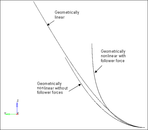
Fig 4: Comparison of deformations for geometrically linear, geometrically nonlinear without application of follower force and geometrically nonlinear analysis with follower force applied
Whether follower force should be applied or not depends on the application. For situations where the applied force rotates with the rotation of the load application point, follower forces should be defined for correct representation of the physical situation. In all other situations where the direction of the force remains constant, follower forces do not need to be considered.


