HMath-4001: Using HyperMath for Material Characterization

HyperMath comes with a powerful curve fitting command to determine the coefficients of an arbitrary function that best fits the supplied data.

This tutorial demonstrates how to calculate the coefficient of a Johnson-Cook material using the NLCurveFit command and a set of experimentally obtained stress and strain data. The file with the target stress and strain data for this problem is the JC_data.txt.

Step 1: Read and plot the the experimental data.

1.	Start HyperMath.

In a new script, type the following commands. The first sets a complete path to the target file that contains the experimental data. Note that the directory path needs to be edited to match the correct installation location on your computer. The second and third commands read the first and second data columns, respectively.

dataFile='C:/Users/JC_data.txt'

strain = ReadVector(dataFile,1,1,1)

stress = ReadVector(dataFile,1,1,2)

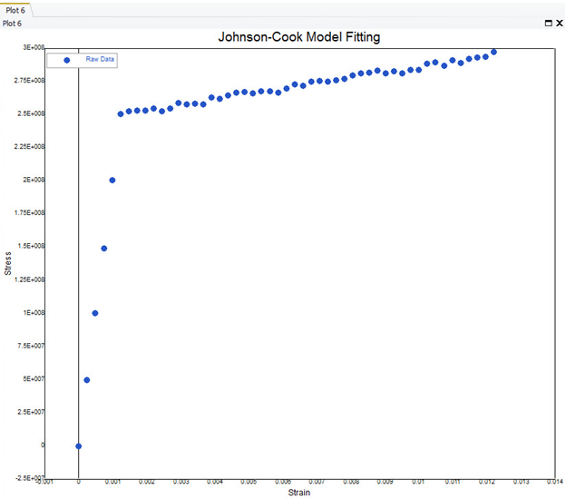
3.	Next, plot the data and set the legend and axis handles using the following commands

DeleteAllPlots()

PlotScatter(strain,stress)

SetLegend('Raw Data')

SetXLabel("Strain")

SetYLabel("Stress")

SetTitle("Johnson-Cook Model Fitting")

LegendPosition('upperleft')

4.	Run the script. The plotted experimental data is displayed as shown below.

hmath_4001_fig1

Step 2: Define the material law expression inside a function.

The command NLCurveFit takes a HyperMath function as an argument. The function has the following requirements:

•	It must take two arguments. The first is a vector of estimates of the parameter values. The second is a vector of the independent data values.

•	It must return the dependant data vector by evaluating the polynomial values at each of the independent data points.

The following code defines a function to evaluate the Johnson-Cook material model. The four material parameters (E, A, B, and N) are passed in the first argument. Observe that the parameters are scaled inside the function. This is done because of the larger differences in scales between parameter values. The goal is to better numerical convergence during the curve fitting.

function JC_fit(values,x)

nn = Length(x)

output = Zeros(1,nn)

E=values(1)*1e9

A=values(2)*1e6

B=values(3)*1e9

N=values(4)

eps_y = A/E

for i = 1,nn do

if (x(i) < eps_y) then

output(i) = E*x(i)

else

output(i) = A + B*(x(i)-eps_y)^N

end

return output

end

Step 3: Create an initial guess and perform the curve fitting.

Because the defined function contains an internal scaling, a good neutral guess is simply "1" for each parameter. These lines of codes create the initial guess, perform the curve fitting, and print the scaled resulting parameters to the HyperMath window. Note that the NLCurveFit command can take additional arguments and return additional values; please see the on-line help for more information on these options.

initial = Ones(1,4)

p=NLCurveFit("JC_fit",initial,strain,stress)

Clc()

print("E=",p(1)*1e9)

print("A=",p(2)*1e6)

print("B=",p(3)*1e9)

print("n=",p(4))s1=[]

Step 4: Plot the best fit curve.

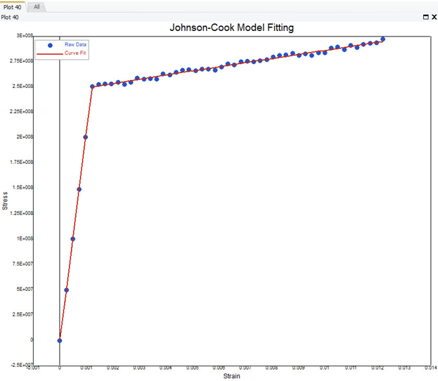
1.	For a final visual inspection, the resulting best fit curve can be plotted against the raw data. The following lines evaluate the function using the best fit parameters and plot the data on the previously existing plot. The results are shown below.

fit=JC_fit(p,strain)

PlotLine(strain,fit)

SetLegend('Curve Fit')

hmath_4001_fig2

HMath-4001: Using HyperMath for Material Characterization

HMath-4001: Using HyperMath for Material Characterization

HMath-4001: Using HyperMath for Material Characterization

See Also: