HMath-4030: Optimization Algorithms in HyperMath

HyperMath can be used to find the optimum of a function f(x) (subject to bounds on the design variables) and constraints using several methods, such as Sequential Quadratic Programming (SQP) and Genetic Algorithm (GA).

This tutorial demonstrates how to optimize a rectangular cross-section cantilever beam, such that the beam volume is minimized while meeting stress requirements. Design Variables are the cross-sectional dimensions (width and height) and the length of the beam.

Step 1: Implement the objective and constraint.

1.	Start HyperMath.

2.	Create a new script and enter the following HyperMath commands to define the objective function and optimization constraints volume and stress, respectively.

function Volume(x)

{

L = x(1)

B = x(2)

H = x(3)

vol = B*H*L

return vol

}

//Setup optimization constraints

function MaxStress(x)

{

L = x(1)

B = x(2)

H = x(3)

P = 100

E = 2e11

M = P*L

c = H/2

I = (B*H^3)/12

str= (M*c)/I

return str

}

Note that each function takes the design variables as an input vector. The order of the variables in the vector is unimportant, but they have to be consistent across the functions, initial values, and the bounds (see below).

Step 2: Define initial values, bounds and constraints.

1.	Define the initial values for the design variables, along with their lower and upper bounds. Also, define the constraint bounds. Note the order of the entries in each vector has to be consistent with the order assumed in the above functions.

init = [100, 5, 10]

lowerBound = [50, 2.5, 5]

upperBound = [100, 5, 10]

conUpBound = [450]

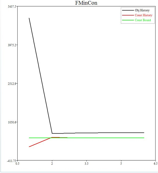
Step 3: Solve the optimization problem using FMinCon.

1.	Solve the optimization problem using FMinCon and plot the iteration histories by adding the following lines:

//Launch FMinCon Algorithm

x,f,c,dh, oh, ch= FMinCon("Volume", "MaxStress", lowerBound, upperBound,conUpBound, init)

2.	The outputs are respectively:

•	A vector of the design variable values at the optimum.

•	The optimum value of the objective.

•	A vector of the constraint values at the optimum.

•	A vector of the design variable history.

•	A vector of the objective function history.

•	A vector of the constraints function history.

3.	We now extract these by adding the following lines:

//Print results to the command window

print("The optimized results are:")

print("Length = ",x[1])

print("Width = ",x[2])

print("Height =",x[3])

print("Volume at optimum = ", f)

print("Max Stress at optimum =", c)

//Plot results

iteration = [1:1:Length(oh)];

ConBound2 = 450*Ones(1, Length(oh))

plot1= PlotLine(iteration, oh, "new")

SetLegend("Obj History")

PlotLine(iteration, ch)

SetLegend("Const History")

PlotLine(iteration, ConBound2)

SetLegend("Const Bound")

SetTitle("FMinCon")

tut_4003_img1

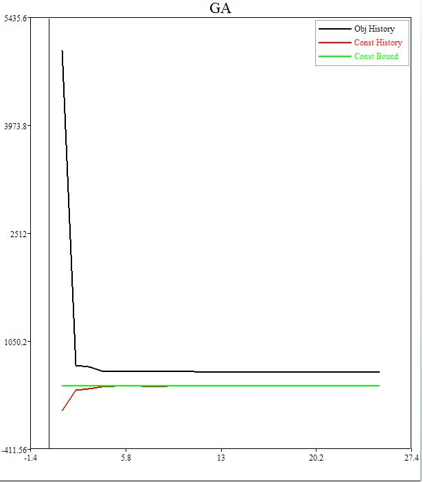
Step 4: Solve the optimization problem using GA.

1.	Solve the optimization problem using GA and plot the iteration histories by adding the following lines:

//Launch GA Algorithm

x,f,c, dh, oh, ch= GA("Volume", "MaxStress", lowerBound, upperBound,conUpBound, init,[],[100] , [50], [3])

2.	The outputs are the same as before. Extract them again by adding the following lines:

//Print results to the command window

print("The optimized results are:")

print("Length = ",x[1])

print("Width = ",x[2])

print("Height =",x[3])

print("Volume at optimum = ", f)

print("Max Stress at optimum =", c)

//Plot results

iteration = [1:1:Length(oh)];

ConBound2 = 450*Ones(1, Length(oh))

plot1= PlotLine(iteration, oh, "new")

SetLegend("Obj History")

PlotLine(iteration, ch)

SetLegend("Const History")

PlotLine(iteration, ConBound2)

SetLegend("Const Bound")

SetTitle("GA")

tut_4003_img2

3.	Quit HyperMath.

HMath-4030: Optimization Algorithms in HyperMath

HMath-4030: Optimization Algorithms in HyperMath

HMath-4030: Optimization Algorithms in HyperMath

See Also: