HMath-4020: Solving Differential Algebraic Equations

When the systems of equations contain both algebraic and ordinary differential equations, it is a differential algebraic equation. The solution method is different than the ordinary differential equations. The differences are in how the user functions are defined and the need for initial conditions for the derivatives of the state variables as well.

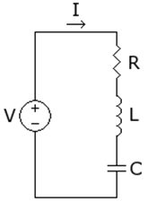
This tutorial will solve the series RLC circuit, subject to an alternating voltage by formulating it as a differential algebraic equation.

tut_4002_img1

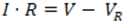
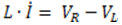
Let:

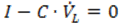
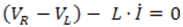
A system of equations representing the circuit is:

Notice that the first equation is a purely algebraic one. The state variables of the system are I, VR and VL. We will attempt to solve for their time-series values.

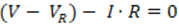
Step 1: Rewriting the equations.

1.	Unlike in ordinary differential equations, for differential algebraic systems, we have to rearrange the equations in terms of residuals:

Step 2: Implementing the two equations.

1.	These equations in the above form need to be implemented in a function of our choice. We will name it RLC_DAE. The function needs to have the following characteristics:

•	Take the current time step point as the first input argument. It is a scalar.

•	Take the current values of the state variables as the second input argument. It is a column vector of length matching the number of state variables in the system (three in our case).

•	Take the current values of the derivatives of state variables as the third input argument. It is a column vector of length matching the number of state variables in the system (three in our case).

•	It must output the residuals in a column vector (in our case, the three equations). The order of the derivatives in the output is arbitrary, but must match the initial conditions when the ODE solver is called.

•	Optionally, it can also take a user defined matrix as the fifth input. We will use it to pass the system constants.

This is what our function looks like:

function RLC_DAE(t, y, yp, userData)

{

// y = [V_R, V_L, I]

// V_R - node voltage between the resistor and the inductor

// V_L - node voltage between the inductor and the capacitor

// I - current

// Extract the system constants from the user data

R = userData(1);

L = userData(2);

C = userData(3);

A = userData(4);

// Now implement the equations

out = Zeros(1,3)

out(1) = (A*Sin(t)-y(1)) - y(3)*R

out(2) = y(3) - C*yp(2)

out(3) = (y(1)-y(2)) - L*yp(3)

return out;

}

Step 3: Using the DAE solver.

1.	For this tutorial, we will use the DAE11a function, specifically its following form:

x = DAE11(func, init, dt_init, time, reltol, abstol, userdata)

where

Option	Description
func	The name of our function we just created.
init	The initial conditions of the state variables, specified as a vector.
dt_init	The initial conditions of the derivatives of the state variables, specified as a vector.
time	The time point where the values of the two state variables are to be calculated.
reltol	Relative tolerance of convergence. We will use the default value of 1e-03.
abstol	Absolute tolerance below which the solutions are unimportant. We will also use the default 1e-06.
userdata	This is a user supplied optional matrix and we will use it to pass the parameter values.
x	A matrix of the solutions at each time point. The columns would represent the state variables.

The initial conditions and the time points where we would like to evaluate the solutions need to be defined. For this example, we would assume the states (voltages and current) and their first derivatives start at zero and create two row vectors of three zeros to represent these (the order of state variable representation in this vector must match the order assumed in the second argument of the function we created). We choose to evaluate the solutions starting from time zero to ten in increments of 0.1. We will also pass in the parameter values as a user defined matrix.

With the above defined, we can simply call DAE11a with our function name, initial condition, and time points. Then, the solver starts the numerical integration, starting with the initial values, calling our function at each time step, passing in the current time, state variable values and their first derivatives, to obtain the corresponding residuals from our function to calculate the next time step values until it reaches the last time point. This all happens behind the scene.

The above can be implemented as follows:

init = [0, 0, 0];

// Initial conditions for the states

dt_init = [0, 0, 0];

// Initial conditions for the state derivatives

params = [1, 1, 1, 1]; // R, L, C & A values

t = [0:0.1:10];

// The time steps for solution

x = DAE11a("RLC_DAE", init, dt_init, t, 1.0e-3, [1.0e-6], params);

The output variable x contains the time-series values for both states. It has three columns and 101 rows. Each column represents a state variable, the first being VR, the second VL, and the third I (consistent with the order assumed in the user function). Each row represents a time-step.

We can extract the current and plot against time as follows:

I = x(:,3); // Extract the circuit current response

PlotLine(t, I,'new');

SetLegend("Current");

SetTitle("DAE Solution");

HMath-4020: Solving Differential Algebraic Equations

HMath-4020: Solving Differential Algebraic Equations

HMath-4020: Solving Differential Algebraic Equations

See Also: