HMath-4000: Using HyperMath Functions for Curve Fitting

In HyperMath, you can write functions to fit equations to data.

This tutorial demonstrates how to use the NLCurveFit and PolyCurveFit commands to fit a polynomial function for a given curve.

Step 1: Solve for the coefficients using the NLCurveFit command.

1.	Start HyperMath.

2.	From the menu bar, select File > Open and locate the Tutorial_CurveFit.hml file, located in the hmath folder. The file looks as shown below:

tut_4000_fig1

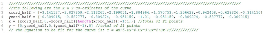
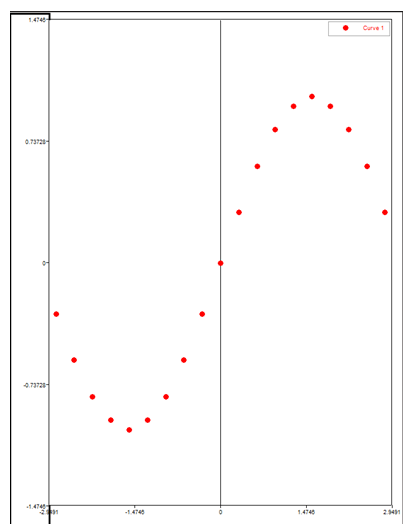
There are 21 points for X and Y coordinates. The data looks like this:

tut_4000_fig2

In the next step, fit a fifth order polynomial to the curve Y = A·x5+B·x4+C·x3+D·x2+E·x+F.

Step 2: Define the polynomial equation inside a function.

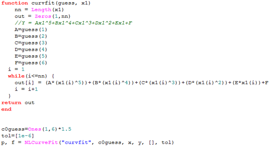
1.	Since the polynomial equation is defined inside a function, HyperMath requires that the function be created before it is invoked from the NLCurveFit command. The function has the following requirements:

•	It must take two arguments. The first is a vector of estimates of the parameter values. The second is a vector of the independent data values.

•	It must return the dependant data vector by evaluating the polynomial values at each of the independent data points.

Add the following lines of code:

function curvfit(guess, x1)

nn = Length(x1)

out = Zeros(1,nn)

//Y = Ax1^5+Bx1^4+Cx1^3+Dx1^2+Ex1+F

A=guess(1)

B=guess(2)

C=guess(3)

D=guess(4)

E=guess(5)

F=guess(6)

i = 1

while(i<=nn) {

out[i] = (A*(x1(i)^5))+(B*(x1(i)^4))+(C*(x1(i)^3))+(D*(x1(i)^2))+(E*x1(i))+F

i = i+1

}

return out

end

The function first determines the length of the independent vector using the Length command. The dependent vector is calculated using the equation for each of the independent vector entries.

Step 3: Setup the NLCurveFit command.

NLCurveFit has the following syntax:

p, r = NLCurveFit(Model, Initial Guesses, Ind Vector, Dep Vector, Max. Iter, Tol)

where:

p – Coefficients of the equation.

r – Quality of the fit.

Model – Above defined HyperMath function containing the polynomial.

Initial Guesses – Initial guess values of the polynomial coefficients.

Ind Vector – X coordinate values (independent data).

Dep Vector – Y coordinate values (observed data).

Max. Iter – Maximum number of iterations performed for searching the best fit (defaults to 200 if empty).

Tol – Tolerance for the iterations. A one-element vector.

1.	Setup the initial guesses to be 1.5 for all parameters:

c0guess=Ones(1,6)*1.5

This creates a vector of six elements with a value of 1.5 each, A=B=C=D=E=F= 1.5.

2.	Set the tolerance value:

tol=[1e-6]

3.	Set up the curve fitting:

p, f = NLCurveFit("curvfit", c0guess, x, y, [], tol)

The finished code should look like the following:

tut_4000_fig3

Step 4: Obtain the coefficients and quality of fit.

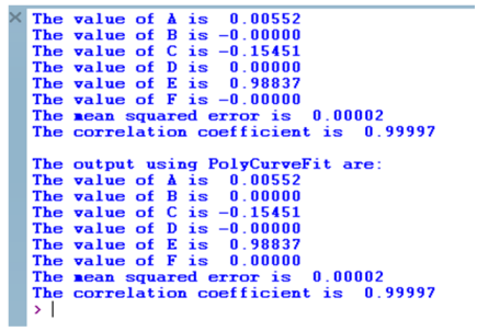
The NLCurveFit command outputs the coefficients for the equation (p) and the quality of the fit. Since there are six coefficients in this equation, the vector "p" has six values containing the values of A through F. The vector "f" always contains two values: Mean squared error (MSE) and Closeness of fit(R^2).

Add the following lines after the NLCurveFit command:

print(string.format("%s %8.5f", "The value of A is", p(1)))

print(string.format("%s %8.5f", "The value of B is", p(2)))

print(string.format("%s %8.5f", "The value of C is", p(3)))

print(string.format("%s %8.5f", "The value of D is", p(4)))

print(string.format("%s %8.5f", "The value of E is", p(5)))

print(string.format("%s %8.5f", "The value of F is", p(6)))

print(string.format("%s %8.5f", "The mean squared error is", f(1)))

print(string.format("%s %8.5f", "The correlation coefficient is", f(2)))

Step 5: Solve for the coefficients using the PolyCurveFit command.

1.	Since we are using the polynomial equation to fit the curve, we could use another command to do the same. The PolyCurveFit command is an easier way to achieve this, since you don't have to provide the initial guesses. The syntax for PolyCurveFit is as follows:

c,s,f = PolyCurveFit(ind vector, dep vector, order of the equation)

where:

c – Coefficients of the polynomial equation.

s – Quality of fit.

Add the following lines:

//Using PolyCurveFit command

c,s,f = PolyCurveFit(x,y,5)

print("\nThe output using PolyCurveFit are:")

print(string.format("%s %8.5f", "The value of A is", c(1)))

print(string.format("%s %8.5f", "The value of B is", c(2)))

print(string.format("%s %8.5f", "The value of C is", c(3)))

print(string.format("%s %8.5f", "The value of D is", c(4)))

print(string.format("%s %8.5f", "The value of E is", c(5)))

print(string.format("%s %8.5f", "The value of F is", c(6)))

print(string.format("%s %8.5f", "The mean squared error is", s(1)))

print(string.format("%s %8.5f", "The correlation coefficient is", s(2)))

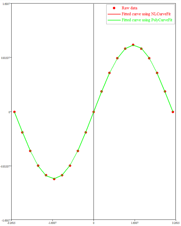
Step 6: Plot all curves.

1.	Next, plot the three curves: the original curve containing the raw data, the curve using the equation from the NLCurveFit command, and the curve using the equation from PolyCurveFit command.

Add the following lines:

PlotScatter(x,y,'new')

SetLegend("Raw data")

y2 = curvfit(p, x)

PlotLine(x,y2)

SetLegend("Fitted curve using NLCurveFit")

y3 = curvfit(c, x)

PlotLine(x,y3)

SetLegend("Fitted curve using PolyCurveFit")

Since the equation is defined in the curvfit function, we pass the coefficients (p and c) and the original independent vector as arguments to the curvfit function and it outputs the dependent vectors (y2 and y3).

Step 7: Execute the file.

1.	Click the Run File icon, , from the toolbar. The command line displays the output as shown and a plot with the fitted curve is also drawn.

tut_4000_fig8

tut_4000_fig9

HMath-4000: Using HyperMath Functions for Curve Fitting

HMath-4000: Using HyperMath Functions for Curve Fitting

HMath-4000: Using HyperMath Functions for Curve Fitting

See Also: