The equivalent static load method has been implemented for the solution of multi-body dynamics problems that include flexible bodies. Size, shape, free-shape, topology, topography, free-size, and material optimization can be applied to flexible bodies. Responses are mass, volume, center of gravity, moment of inertia, stress, strain, compliance (strain energy), and displacement of the flexible bodies. Displacement responses are taken into account with respect to local boundary conditions defined on the flexible body (see definition below). Responses are defined using DRESP1, DRESP2, and DRESP3 bulk data entries. Responses can only be defined on flexible bodies (PFBODY) using the properties, elements and grid points included in such bodies as reference. Design variables are defined using DESVAR, DVPREL1, DVPREL2, DVMREL1, DVMREL2, DSHAPE, DTPL, DTPG, DSIZE, and DVGRID bulk data entries. Free-size optimization is currently only available when PTYPE=PSHELL on the DSIZE card. Design variables can only be defined on flexible bodies (PFBODY) using the properties included in such bodies as reference. Constraints are defined using DCONSTR, DCONADD and DOBJREF bulk data entries. Constraints and objectives are referenced in the multi-body dynamics subcase or globally through DESOBJ, DESSUB, DESGLB, and MINMAX, respectively.

ESLM specific parameters can be set through the DOPTPRM bulk data entry (Parameters for the ESLM).

The Method

---

An optimum solution can be found through a series of static response optimizations with the equivalent static load set, that is:

Where, feq, u, a, v, and f are the equivalent static load, deformation, acceleration, velocity, and external load, respectively. The steps involved in the ESLM can be summarized as:

The iteration at the third step is referred to as an inner iteration; Steps 2 through 4 form the outer loop. The converged solution at Step 3 is the starting point of the next outer loop (if the design does not converge at the current outer loop). If there are time steps in the multi-body dynamics analysis at Step 2, subcases in static response optimization are generated at Step 3 (provided that the time step screening option is deactivated). See Parameters for the ESLM.

 

Boundary Conditions for Structural Analysis and Optimization

---

To perform structural optimization with ESL, you must specify boundary conditions for each flexible body. In the solution of the dynamic analysis, the flexible and rigid bodies are connected by joints to form a multi-body system. When performing ESLM on the flexible bodies, these joints are not included in this static subcase-based structural optimization. This means that each flexible body will have 6 rigid body modes. The 6 rigid body modes of each flexible body must be removed for structural analysis. Exactly 6 degrees of freedom (DOF) of each flexible body must be fixed to remove the 6 rigid body modes. If more than 6 DOF are fixed in a flexible body, the additional fixed DOF become the constraint of the flexible body, which may not result in an optimal solution and consequently increases the required ESLM outer loops.

Due to the way ESL is calculated, each flexible body is in its equilibrium at the 0-th inner iteration of each outer loop. This is why you can fix an arbitrary 6DOF (usually single node) to get rid of rigid body modes in order to do static analysis with ESL. Reaction force at the fixed node is zero at the 0-th inner iteration. Thus, no additional load is applied to a flexible body although 6DOF of the flexible body are fixed. However, design changes occur as the inner iteration goes on. This means the original configuration that maintains equilibrium also changes. As a result, the equilibrium status does not hold true anymore from the 1st inner iteration in each outer loop. An undesirable effect caused by a broken equilibrium status (disequilibrium status) is the reaction force at the fixed point is not zero anymore, which means additional load is applied to that fixed point. This effect, due to shape/size changes, can be minimized by fixing a proper node, as explained below.

A common way to remove the 6 rigid body modes is to fix all 6 DOF of a node. When looking for a node to fix, choose one that is not in a high stress region. If the fixed point is located in a high stress region, the optimization can be very slow. It is highly recommended that the 6 DOF of an independent node of a spider or rigid element (usually used to model joints) be selected to be fixed. On solid models, where the nodes do not have rotational stiffness; if a solid model does not have a rigid element to represent a joint, the next best way to remove the 6 rigid body modes is to fix 3 translational DOF (123) of one node, 2 translational DOF (23) of another node, and 1 translational DOF (3) of a third node. However, still make sure that the 3 nodes are not in a high stress region, otherwise this method of removing 6 rigid body modes does not work. One way or another, all of the 6 rigid body modes of each flexible body must be removed. SPC, SPC1, or SPCADD (referenced in the Subcase Information section) can define the fixed DOF.

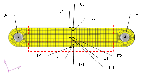
Solid model with joints at the centers of two holes.

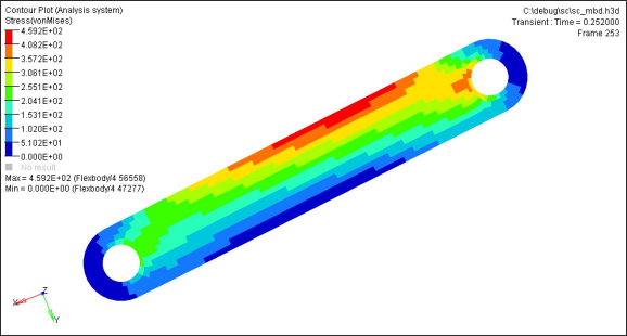
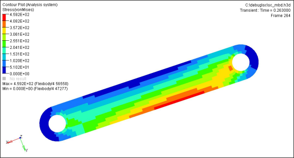
Stress contours of this model at two time steps are shown in the following images.

Nodes A and B are the locations of joints. The best option here is to fix 6 DOF of either node (A or B) in order to remove 6 rigid body motions in this model. To fix alternative nodes other than node A or B, it would work to fix 3 DOF (123) of node E1, 2 DOF (23) of node E2, and 1 DOF (3) of node E3. These three nodes are located in a relatively low stress region. In this model, nodes C1, C2, and C3 or nodes D1, D2, and D3 would take a long time to converge if fixed. Again, the best and simplest way to remove 6 rigid body modes of each flexible body is to fix one of the joint locations in each flexible body.

When the boundary conditions are properly defined, displacement constraints in an optimization can be applied to limit the deformation of the flexible body. An example is to optimize a rotating cantilever, by fixing either the left end or the middle point to retrieve deformation as long as the point has nothing or little to do with the shape perturbation vectors. If a relative displacement at the right end with respect to the left end is to be constrained, it would be most convenient to fix the 6 DOF of the left end to measure the relative displacement. Constraining a relative displacement of the left end with respect to the middle point of the cantilever, it would be best to fix the 6 DOF of the middle point. Regardless of whether the left end or the middle point (or even the right end) is fixed, the stress is the same. If the optimization problem is simply to constrain stress or minimize the maximum stress of a flexible body, all that is needed is to fix one proper node of the flexible body.

Rotating cantilever

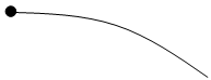
Deformation when the left end is fixed

Deformation when the middle point is fixed

Output Files Generated by the Optimization Process

---

Once ESL optimization converges, the following output files are available:

In addition to the above output files, .desvar, .prop, .grid, .fsthick, and .oss will be found, if available.

See Also:

Convergence Enhancement for the ESLM

Output Requests and ESLM

MBD System Level Response Optimization