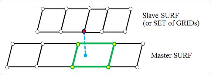
Contact between the master and slave surfaces can be constructed through two main approaches. This process is called discretization, and it defines the basic structure of the contact elements that are constructed to handle the contact condition. They are as follows:

Node-to-Surface Discretization

The Node-to-Surface Discretization approach involves the creation of contact elements linking the Master Surfaces to Slave Nodes. The contact interface is constructed by searching, for each slave node, a respective facet of the master surface, which contains the normal projection of the slave and is within the Search Distance (SRCHDIS field on the CONTACT entry) distance from the slave node.

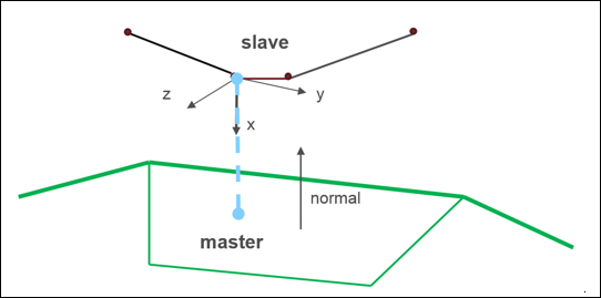
Structure of an N2S Contact Element.

One slave node

A few master nodes

One master face including the master nodes

One projection from the slave node to the master face

For each slave node, a respective master segment will be looked for, which contains the normal projection of the slave and is within SRCHDIS (CONTACT or TIE entry) distance from the slave node.

If a master segment with normal projection is not found, the nearest segment is selected, if the direction from the slave to master is within a certain angle (30 degrees) relative to the normal to the master segment.

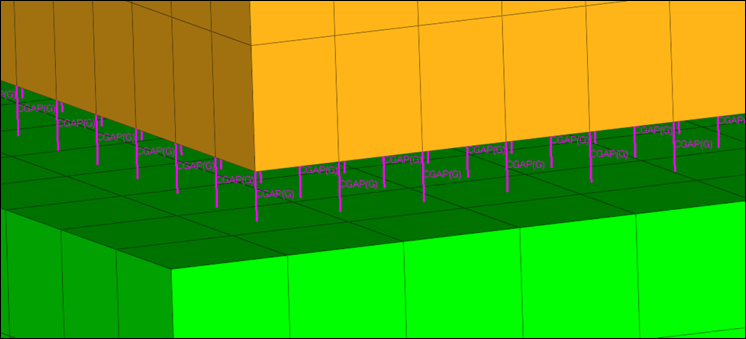
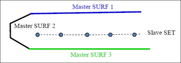
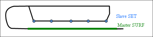
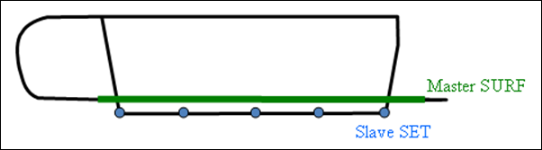
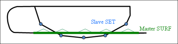
Presently one CONTACT/TIE element is created for each slave node. This assures reasonably efficient numerical computations without creating an excessive number of contact/tie elements. However, this may require special handling in some cases, such as when a master surface wraps around the slave set. In such cases, switching the role of slave and master may be recommended. Alternatively, multiple CONTACT/TIE interfaces can be created in order to cover all possible directions of relative motion (below is a simplified illustration). Additionally, individual GAP(G) elements can be used to handle such special situations.

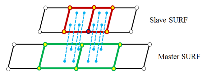
Special case - Master surface wraps around a slave node set

Surface-to-Surface Discretization

The Surface-to-Surface Discretization approach involves the creation of contact elements linking the Master Surfaces to Slave Surfaces. The contact interface is constructed by searching, for each facet of the slave surface, respective facets of the master surface, which contains the normal projection of sample points on the slave facets and is within the Search Distance (SRCHDIS) distance from the sample points. For a slave node, a contact element is created with the surrounding slave facets and the master facets found by projection of the sample points on the slave facets.

The structure of Surface-to-Surface contact elements is different when compared to that of the Node-to-Surface (N2S) CGAP(G) elements.

One core slave node

Several slave nodes surrounding the "core" slave node

One or more slave faces including the slave nodes and sharing the "core" slave node

Several master nodes

One or more master faces including the master nodes

One or more projections from the slave faces to the master faces

For each slave facet, a respective master facet will first be searched which contains the normal projection of the sample points on the slave facet and is within the SRCHDIS distance from the sample points. Then, for each slave node, the contact element is created with the surrounding slave facets and the master facets found by projection of the sample points on the slave facets.

CONTPRM,CONTOUT,YES can be used to visualize S2S contact elements (and large-displacement N2S contact elements) as PLOTEL+RBE3 elements. The *.contout.fem file contains the elements for visualization only.

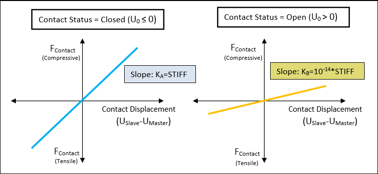
Discretization of the contact interface into contact elements is the initial step towards incorporating the effect of contact in the solution process. These contact elements are then automatically assigned attributes used to define the behavior of the contact interface, including the effect of the contact on the stiffness, boundary condition, and force matrices in the FEA solution. The following approaches are available:

Penalty-based Contact

The majority of contact implementation within OptiStruct involves the penalty-based process. This can be activated using the CONTACT (PCONT, if necessary) and TIE Bulk Data Entries. The TIE entry supports both Penalty-based and Lagrange Multipliers-based formulations. Both Node-to-Surface (N2S) and Surface-to-Surface (S2S) discretization methods utilize this process to implement contact between parts. The discretized contact elements are assigned variable stiffness values (penalties) depending on the proximity of the contact surfaces to each other and the type of contact forces on the element. The primary purpose of the variable stiffness values is to minimize penetration of the contact surfaces.

The stiffness of each contact element typically depends on the type of analysis, linear or nonlinear, that is being performed. For Linear Analysis, the contact stiffness is constant throughout the solution. The contact stiffness depends on the initial state of the contact. If the contact is initially open, it remains open for the duration of the run. The same goes for closed contacts. The contact status or the contact stiffness values are not updated during the course of the solution for linear runs. The initial contact stiffness of each contact element depends on the initial contact gap opening distance (U0), which is calculated based on the positions of the Slave and Master (including contributions from the GPAD field, if any). For open contact elements, a very small stiffness value of KB=10-14 * STIFF is used to avoid numerical singularities.

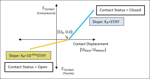
Penalty-based Contact element Force-Displacement curves for Linear Analysis.

Linear penalty curve (Nonlinear analysis)

For Nonlinear Analysis, the contact status can change during the run, which implies that the contact element stiffness can switch between the closed (KA) and open (KB) values. For nonlinear analysis, the contact condition does not change within an iteration, during reevaluation at the end of each iteration, if the contact condition for some or all contact elements has changed, the revised contact condition is used for the subsequent iteration. Therefore the over the course of a nonlinear analysis the contact can open or close multiple times. The Contact stiffness is KA when closed and KB when open, similar to the linear case; however, since the contact status can change, the Contact element force is not tensile, with slope KA, when the contact moves from closed to open status. When the contact is open, the normal stiffness is essentially zero (very small slope KB to avoid singularities). The closure of the contact element increases the stiffness value to KA.

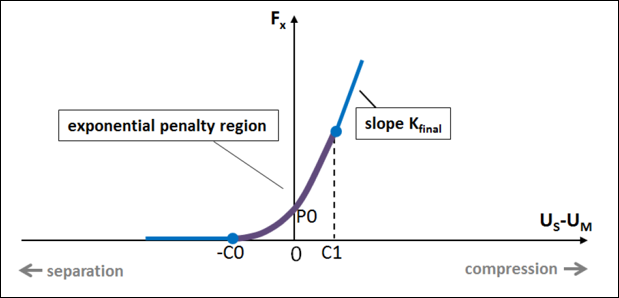
Penalty-based Contact element Force-Displacement curves for Nonlinear Analysis.

The STIFF field on the PCONT Bulk Data Entry can be used to control the stiffness of the contact interface. The AUTO, SOFT, and HARD options are available for automatic predefined stiffness setting. Additionally, a positive real value can be specified to directly prescribe the contact stiffness value. If a negative real value is specified, then it scales the STIFF=AUTO value by the specified scaling factor.

Nonlinear penalty curve (Nonlinear Analysis)

In the previous section, Linear penalty curve was discussed, wherein, the contact stiffness remains constant when either in the open or closed configuration, and only changes when the contact status is updated. This may, in some small number of cases, lead to convergence difficulties due to the sudden and highly discontinuous nature of the stiffness change. To help smooth the stiffness change at the contact open/close location, nonlinear penalty curves can be used via the STFEXP and STFQDR continuation lines on the PCONT entry. Nonlinear penalty curves are currently only applicable to S2S contact discretizations.

Exponential nonlinear penalty

The exponential nonlinear penalty curve has three regions, as shown below. For S2S contact, the force Fx in the figure denotes contact pressure.

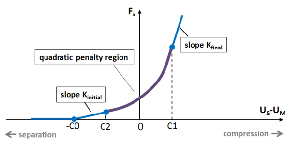
C0 and P0 are specified on the corresponding fields in the STFEXP continuation line. Kfinal and C1 are automatically determined by the C0, P0, and the STIFF fields.

Quadratic nonlinear penalty

The quadratic nonlinear penalty curve has four regions, as shown below. For S2S contact, the force Fx in the figure denotes contact pressure.

C0, ALPHA1, ALPHA2, and ALPHA3 are specified on the corresponding fields in the STFQDR continuation line. Kfinal is automatically determined based on the STIFF field. C1, C2, and Kinitial are defined as follows:

ALPHA1 = C1/ (Characteristic Length)

ALPHA2 = (C2 + C0)/(C1 + C0)

ALPHA3 = Kinitial/Kfinal

The exponential and quadratic nonlinear penalty definitions are currently not applicable to FREEZE contact. They are also ignored for contacts in linear analysis.

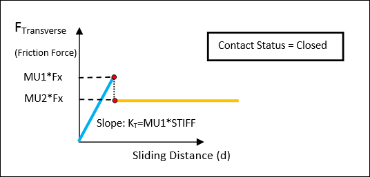
Friction

In real-world applications, a majority of contact-based systems are affected by friction-induced shear stresses to varying degrees. Frictional effects occur when two surfaces come into contact and try to move tangentially relative to one another. A variety of factors affect the amount of friction that exist between the surfaces. Friction is a function of the nature of the surfaces in contact (coefficient of static and kinetic friction) and the normal reaction at the contact interface (Normal force). It is a highly nonlinear problem in finite element analysis, and should be utilized only if the inclusion of frictional effects is essential to the solution of the problem. The MUMPS solver is used in models involving friction. Friction effects generate unsymmetrical terms when surfaces slide relative to one another. These terms may have a strong influence in the overall displacement field. The unsymmetric solver (MUMPS) will be used by default when friction is specified. This may lead to slower convergence, however the results are accurate. The MUMPS solver can be turned off if frictional effects are not anticipated to be significant using PARAM,UNSYMSLV,NO.

Friction can be incorporated within the OptiStruct contact interface in two ways. The MU1 (and/or MU2) field on the PCONT Bulk Data entry, or MU1 field on the CONTACT Bulk Data Entry. For Geometric Nonlinear Analysis (RADIOSS Integration), the FRIC field on the PCONTX/PCNTX# entries can be used. If these fields are not set, then the friction value on MU1 field on CONTACT/PCONT is used.

OptiStruct uses the Isotropic Coulomb Friction model to solve the friction problem. Based on the Isotropic Coulomb Model, friction, in the real world, can be idealized as an increasing force with zero tangential slip up to the static friction limit. Then sliding is initiated and the frictional force immediately switches to the kinetic friction force. However, in the finite element analysis, such idealization can lead to convergence difficulties due to the presence of extreme discontinuities. Therefore, a nonlinear spring model is used, wherein the transverse frictional force increases linearly with the sliding distance until it reaches the static frictional limit, and then switches to the kinetic frictional force which is constant afterwards. The stiffness of this spring is equal to KT=MU1*STIFF (KT=0.1*STIFF in the case of STICK) in the transverse direction until the static limit is reached. This acts as a linear spring in linear solution sequences. For nonlinear solution sequences, the frictional force increases with sliding distance in proportion to KT until it reaches the static frictional limit force (MU1*Fx), where Fx is the normal force in the contact element. With further transverse deformation, friction becomes kinetic and the frictional force is MU2*Fx.

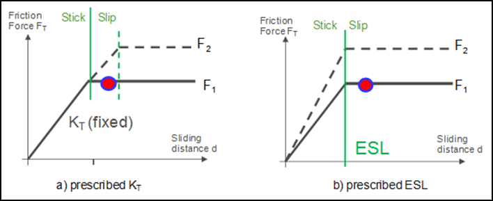
Note that the nonlinear contact element’s force-displacement behavior may produce negative contributions to the compliance of the structure. As an example, when slave and master bodies have initial overlap and the contact releases elastic energy during the solution.

Friction Models

Two models of friction are available in nonlinear analysis:

The latter model typically has better performance in solution of frictional problems, due to stable handling of transitions from stick to slip. The key differences between the two available models are illustrated below (F1 and F2 represent two different values of normal force Fx):

Comparison of the two friction models for contact elements.

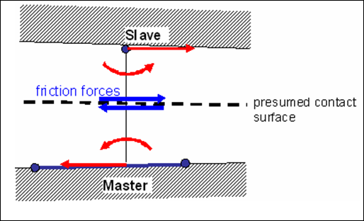
The model (b), which is currently the default, is recommended for solution of nonlinear problems with friction. For backward compatibility, the model based on fixed KT can be activated by setting FRICESL=0 on PCONT or CONTPRM entries.

For Small Sliding, the frictional force is always directed back to the point where the slave and master first came into contact (changed status from open to closed). Its location is estimated using proportional interpolation between the current position and the last converged solution before penetration.

The presence of friction can introduce moment loadings and counter-intuitive results into the problem by way of frictional offset. The reason for this is that, for contact elements with non-zero length (distance between slave node and master segment), the actual location of the contact interface is presumed to be in the middle of the contact element’s length, shown below.

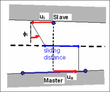
CONTACT presumed contact surface

The frictional forces act along this contact surface. Transferring these forces to the slave and master objects requires an offset operation that produces both forces and moments at slave and master. Similarly, the sliding distance at the contact interface is a result of nodal displacements and rotations of the slave node and master segment, shown below.

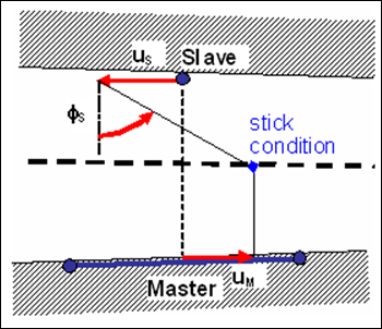
CONTACT sliding with friction

Master segments, which consist of several nodes, can effectively resist these offset forces and moments. However, for slave bodies that do not support moments (nodes of solid elements, for example), this offset may render friction ineffective because the free rotations at slave nodes offer no effective resistance to friction. With the stick condition formally satisfied, for example, slave and master can move relative to each other, shown below.

CONTACT stick (zero sliding distance)

In practice, for contact interfaces that are initially open, AUTOSPC will effectively fix respective unsupported rotations. However, for contacts that are initially closed (for example, pre-penetrating contact with MORIENT=NORMAL) the frictional terms will prevent AUTOSPC from being effective. Therefore, respective SPC on rotations need to be applied manually to respective slave nodes.

To avoid such counter-intuitive behavior, effective in Release 12.0, the frictional offset operation is turned off by default, if the model involves friction or stick and contains at least one nonlinear subcase (of NLSTAT type). (Note that for consistency, this affects both linear and nonlinear contact elements.) This produces more intuitive results with friction; however, it may violate the rigid body balance of the body.

The above default setting can be changed using GAPPRM,GAPOFFS.

The presence of friction, due to its strongly nonlinear, non-conservative nature, may cause difficulties in nonlinear convergence, especially when sliding is present. If frictional resistance is essential to the solution of the problem and convergence problems are encountered, enforcing the stick condition (by setting KT>0 and MU=0) may be a viable solution that will often result in better convergence than with Coulomb friction. Note however, that this only applies to problems in which minimal sliding is expected. In the case of larger sliding motions, the stick condition may lead to divergence through a “tumbling” mode.

Lagrange Multipliers (MPC-based)

MPC-based contact utilizes multi-point constraints (MPC’s) to define a tied contact between the master and slave surfaces. It is activated using CONTPRM,TIE,MPC and TIE Bulk Data entries. All TIE contacts in the model are defined using the MPC-based method. This method uses Lagrange Multipliers and is not applicable to CONTACT bulk data entries of TYPE=FREEZE.

Fast Contact (SUPORT-based and CONTACT/CGAP(G)-based)

Fast Contact uses a different formulation when compared to the Penalty-based approach and the SUPORT-based contact. This is applicable in cases where the only nonlinearities in the model arise due to Contact and the model includes small deformations and small sliding. This is also not applicable to Large Displacement Nonlinear Analysis (LGDISP). There are two approaches to Fast Contact in OptiStruct, SUPORT-based and CONTACT/CGAP(G)-based.

SUPORT-based Fast Contact

If the only nonlinearity in the model is contact between parts and if the deformation at the contact interface resides within the small-displacement domain, SUPORT-based Fast Contact can be used to setup a linear solution using SUPORT and PARAM, CDITER. Optionally, MPC’s, SUPORT and SPC entries can be used.

Note: MPCs are optional for SUPORT-based contact. For example, if the initial gap is required (using SPCs,) then MPCs, SPCs and SPOINTs are required.

Contact elements are not constructed, thereby avoiding the nonlinearities inherent in the penalty-based contact. The process involves applying constraints to grid points.

The penetration between the parts is avoided by limiting the relative displacement component in the normal contact direction at the contact interface to a positive value. Additionally, the force at the contact interface is also limited to a positive value, which avoids tension forces.

For SUPORT+MPC contact, the process initially assumes all contacts to be closed regardless of the position of the master and slave. For SUPORT only contact, the initial contact status is all open. Then OptiStruct applies the constraints in an iterative process to avoid both penetration and tensile forces. An initial starting point depicting the contact status as 0.0 (open) or 1.0 (close) using DMIG, CDSHUT can also be provided (CDSHUT is supported only for SUPORT+MPC contact).

The performance of Fast Contact is dependent on the initial gap status. For example, if only a small number of contact is to be closed at the end of analysis, it is better to start the analysis with all gaps to be open (making sure the sufficient support is provided to hold the parts together even in that condition).

Setting up the MPC equation

MPC Equation

Example Input Deck

CONTACT/CGAP(G)-based Fast Contact

CONTACT/CGAP(G)-based Fast Contact is an alternative approach to Fast Contact when compared to the SUPORT-based Fast Contact. The main advantage of this approach is that MPC equations, SUPORT’s, SPC’s are not required. Instead, the process of Contact Interface setup is exactly the same as in the case of the Nonlinear Static Analysis. The Contact Interface can be defined using the CONTACT Bulk Data Entry, with Node-to-Surface (N2S) discretization to generate the contact elements (Surface-to-Surface S2S discretization is not currently supported). OptiStruct then uses a new iterative approach to resolve the contact situation. The same limitations that apply to SUPORT-based Fast Contact also apply to CONTACT/CGAP(G)-based Fast Contact. Additionally, only sliding contact without friction is currently supported. Also, no nonlinear material and geometric nonlinearity are allowed.

It is activated by simply adding PARAM,FASTCONT,YES in a model that contains a predefined contact interface.

Initial gap opening will be specified by U0 on PGAP and CLEARANCE on PCONT or CONTACT bulk entry.

The next step after the contact interface is generated, contact elements are properly discretized, and the contact implementation type is selected as per the requirements of the problem, is the selection of the Contact Interface Type. This depends on the behavior being simulated at the contact interface.

Freeze Contact

Freeze Contact enforces zero relative motion on the contact surface, the contact gap opening remains fixed at the original value and the sliding distance is forced to be zero. Additionally, rotations at the slave node are matched to the rotations of the master patch. The FREEZE condition applies to all respective contact elements, regardless of whether they are open or closed. Freeze Contact can be activated using TYPE=FREEZE on the CONTACT, MU1=FREEZE on the PCONT entry or by using the Penalty-based Tied Contact. Penalty-based tied contact is activated by using the TIE entry for the contact interface (with CONTPRM,TIE,PENALTY, the default).

Sliding Contact

Sliding Contact has only normal contact stiffness at the contact interface and no frictional effects. It is only valid for small sliding without friction and applies to both open and closed contacts. If convergence difficulties arise, adding a small value of friction may help, or the STICK condition can be used. Sliding Contact can be activated using TYPE=SLIDE on the CONTACT entry.

Stick Contact

Stick contact is an enforced stick condition, wherein such contact interfaces will not enter the sliding phase. It only applies to contacts that are closed. Note that, in order to effectively enforce the stick condition, frictional offset may require to be turned off. Stick contact is activated using TYPE=STICK on the CONTACT entry or MU1=STICK on the PCONT entry. The contact stiffness value (KT) is equal to 0.1*STIFF in the case of Stick Contact.

Frictional Contact

For detailed information, refer to Friction.

Thermal Contact

For detailed information, refer to Thermal Contact in the User's Guide.

Fast Contact

For detailed information, refer to Fast Contact.

Orientation of contact pushout force (MORIENT)

The orientation of the contact pushout force from the master surface can be defined on the MORIENT field on the CONTACT entry. It applies only to masters that consist of shell elements or patches of grids. Masters defined on solid elements always push outwards irrespective of this flag. MORIENT is the direction of contact force that master surface exerts on slave nodes.

It is important to note that, in most practical applications, leaving this field blank will provide correct resolution of contact, irrespective of the orientation of surface normals. Only in cases of master surfaces defined as shells or patches of grids, and combined with initial pre-penetration, is MORIENT needed.

By default, MORIENT is ignored for solid elements – it applies only to master surfaces that consist of shell elements or patches of grids. Master surfaces defined as faces of solid elements always push outwards, irrespective of the surface normals, or whether the contact gap is initially open or closed.

Example for the use of OPENGAP

Example for the use of OVERLAP

Example for the use of NORM

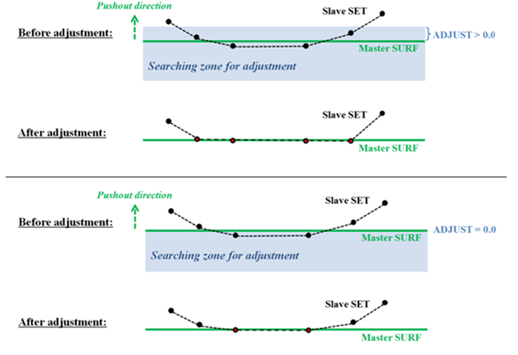
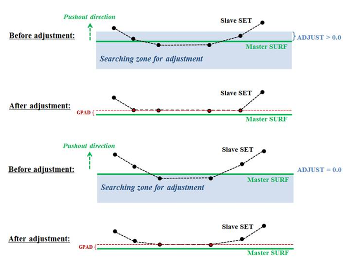
By default, MORIENT does not apply to masters that are defined on solid elements – such masters always push outwards. This can be changed by choosing CONTPRM,CORIENT,ONALL which extends the meaning of MORIENT to all contact surfaces. In which case, it should be noted that the default normal is pointing inwards unless a FLIP flag appears on the master SURF definition for surfaces on solid elements, making the surface normal point outwards. (When creating contact surfaces in HyperMesh, this behavior corresponds to that of the reverse normals checkbox on the contactsurfs panel).

Search Distance (SRCHDIS)

The SRCHDIS field on the CONTACT and TIE entries is the search distance criterion for creating the contact interface. When specified, only slave nodes that are within the SRCHDIS distance from the master surface will have the contact condition checked. The default value is equal to twice the average edge length of the master surface. For FREEZE contact, it is equal to half the average edge length.

Contact Adjustment (ADJUST)

Contact Adjustment can be used to adjust the slave nodes onto the master surface at the beginning of the run. The ADJUST field on the CONTACT and TIE entries can be used, with the available options:

NO – no adjustment (default).

AUTO – A real value equal to 5% of the average edge length on the master surface is internally assigned as the depth criterion.

Real > 0.0 – value of the depth criterion which defines the zone in which a search is conducted for slave nodes (for which contact elements have been created). These slave nodes (with created contact elements) are then adjusted onto the master surface. The assigned depth criterion is used to define the searching zone in the pushout direction.

Integer > 0 – identification number of a SET entry with TYPE = GRID. Only the nodes on the slave entity which also belong to this SET will be selected for adjustment.

The adjustment of slave nodes does not create any strain in the model. If DISCRET=N2S is selected, it is treated as a change in the initial model geometry. If DISCRET=S2S is selected, it is treated as a change in the initial contact opening/penetration.

If a node on the slave entity lies outside the projection zone of the master surface, it will always be skipped during adjustment since no contact element has been constructed for it.

Contact interface padding, GPAD (on the PCONT entry) is used to determine the direction and distance of slave node adjustment, not to decide if a particular node will be adjusted. If the MORIENT field is OPENGAP or OVERLAP while the GPAD field in the referred PCONT entry is NONE or zero, the nodal adjustment will be skipped, since for OPENGAP or OVERLAP there is no way to decide the master pushout direction if slave nodes are adjusted to be exactly on the master face.

If different contact interfaces involve the same nodes, nodal adjustment definitions are processed sequentially in the order of identification numbers of the contact interfaces. Care must be taken to avoid conflicts between the nodal adjustments; otherwise, contact element errors or lack of compliance may occur.

a) The ADJUST field must be set to NO for self-contact.

b) If a real value (the searching depth criterion for adjustment) is input for the ADJUST field, a searching zone for adjustment is defined. The slave nodes in this searching zone, for which contact elements have been created, will be adjusted. If ADJUST is larger than or equal to SRCHDIS, all the slave nodes for which contact elements have been created, will be adjusted.

No Contact Interface Padding (GPAD):

With Contact Interface Padding (GPAD):

An illustration depicting how ADJUST works.

c) If the ADJUST field is set to an integer value (the identification number of a grid SET entry), the nodes shared by the slave entity and the grid SET will be checked for contact creation, that is, SRCHDIS will be ignored for these nodes, and then adjusted if a projection is found. The nodes belonging to the grid SET but not to the slave entity will be simply ignored.

Contact Clearance (CLEARANCE)

Clearance can be defined on the CONTACT or PCONT entries on the CLEARANCE field. It can also be defined via U0 on the PGAP entry. Clearance does not physically move the nodes. The contact is considered to be closed, if the clearance between the two surfaces is equal to (or less than) the specified clearance, regardless of the physical location of the nodes. Make sure that the surface nodes are not highly irregular or the actual physical distance between some (or all) parts of the surfaces is much greater than the specified clearance. The resulting contact parameters applied to the actual physical nodes after each iteration or over the entire solution may be inaccurate in such cases. A blank clearance field is the same as U0 = AUTO.

Using CLEARANCE overrides the default contact behavior of calculating initial gap opening from the actual distance between Slave and Master. CLEARANCE is now equal to the distance that Slave and Master have to move towards each other in order to close the contact. Negative value of CLEARANCE indicates that the bodies have initial pre-penetration.

Contact smoothing (SMOOTH)

Optional SMOOTH continuation line(s) is used to define contact smoothing for region(s) of master and/or slave surfaces.

Finite Sliding (TRACK)

Finite Sliding (TRACK=FINITE or CONSLI) option is currently supported only if TYPE=SLIDE or if friction (via MU1/CONTPRM/PCONT) is defined.

For TRACK=FINITE, the contact search is conducted for every load step, while with TRACK=CONSLI, the search is done for every iteration. The CONSLI option is expected to produce more accurate results and in some cases, better convergence robustness, especially when very large sliding and/or distortion is present.

For non-solid elements, the MORIENT field should not be set to OPENGAP or OVERLAP for Finite Sliding. If CONTPRM,CORIENT,ONALL is active, MORIENT is applied to solid elements. In such cases, MORIENT should not be set to OPENGAP or OVERLAP for solid elements also.

To activate Finite Sliding, it is important to review the following:

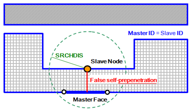
Contact Interface Padding (GPAD)

“Padding” of the interface to account for additional layers, such as shell thickness. This value is subtracted from the contact gap opening as calculated from the location of nodes. It is set on the GPAD field of the CONTACT and PCONT entries. CLEARANCE cannot be set in conjunction with (non-zero) GPAD. Blank GPAD field in presence of CLEARANCE is interpreted as NONE.

The initial contact gap opening is calculated automatically based on the relative location of slave and master nodes (in the original, undeformed mesh). To account for additional material layers covering master and slave objects, the GPAD entry can be used. GPAD option THICK automatically accounts for shell thickness on both sides of the contact interface (this also includes the effects of shell element offset ZOFFS or composite offset Z0), when the master and/or slave are shell surfaces (SET of shell element types or SURF of shell element faces). The THICK option will only apply automatic padding if shells are selected for master/slave in the contact interface (for example, padding is not applied for “skinned” solid elements that are selected as a master/slave in the contact interface).

Contact Stabilization (CNTSTB entry and PARAM,EXPERTNL,CNTSTB)

Defines parameters for stabilization control of surface-to-surface contact and large displacement node-to-surface contact. A CNTSTB Bulk Data entry should be referenced by a CNTSTB Subcase Information entry to be applied in a particular subcase. Also, PARAM,EXPERTNL,CNTSTB can be used to apply contact stabilization.

Resolution of Pre-penetration (CONTPRM,SFPRPEN)

The CONTACT capability in NLSTAT solution is designed to correctly resolve initial pre-penetration, such as happens in press fit, and so on. This usually works reliably with correct identification of Master and Slave surfaces. However, in some cases contact surfaces by property are created for convenience, which results in contact surfaces enveloping the entire solid bodies. Also, the Slave and Master could receive the same ID, which is known as self-contact (not recommended, in spite of the convenience factor). In such cases, it is possible to encounter false self-penetrations, as illustrated below:

In the case above, the Slave node will be identified as if pre-penetrating the Master face, while in reality it is on the other side of the same solid body. The result from nonlinear CONTACT solution will be such that this portion of the body will be “squeezed” to have practically zero thickness, with very high stresses obviously resulting.

Apart from correctly identifying potential Slave and Master sets, a possible remedy to avoid such situations is to make sure that SRCHDIS is smaller than minimum thickness of the solid bodies which are enveloped by self-contacting surfaces.

An alternative, viable when there are no actual pre-penetrations in the problem, is to choose SFPRPEN = NO, which will ignore initial pre-penetrations on self-contacting surfaces (some minor pre-penetrations, due to variations of nodal positions will still be correctly resolved – up to the minimum element size on the respective contact surfaces).

Note that SFPRPEN affects only surfaces that actually have self-penetration, as in a case where the Slave Node and Master Face belong to the same contact set or surface. On properly defined, disjoint Slave and Master surfaces, the initial pre-penetrations will be resolved irrespective of this parameter.

Contact Friendly Elements (CONTFEL)

Contact friendly elements can be activated using PARAM,CONTFEL,YES. Contact-friendly TETRA10, HEXA20, and PENTA15 elements are available and can be combined in a single model. Modified shape functions are used for possible improved runs with contact friendly elements.

No Separation Contact (SEPARATION)

Flag indicating whether the master and the slave can separate once the contact has been closed. This is set on the PCONT Bulk Data Entry, via the SEPARATION field. If SEPARATION is set to NO, then the master and slave do not separate after contact is closed. Applied only to frictional, SLIDE and STICK contacts with S2S or large-displacement N2S.

Based on the various contact properties and implementations, the following special or dedicated Contact Applications are available in OptiStruct:

Pretensioned Bolt Analysis

If the master facet of a contact projection includes a grid on any pretension cutting surface, this contact projection will be included for consideration of contact. For additional detailed information, refer to Pretensioned Bolt Analysis in the User's Guide.

Optimization with Contact

All Optimization types and all responses (wherever applicable) are available for optimization when contact is present. Topology, Topography, Size, Shape, Free-Shape, and Free-Size optimization types are all supported. Freeze contact with large shape changes is available for optimization.

Large Displacement Nonlinear Analysis with contact is not supported for optimization. Stress/Strain responses when plasticity is involved is not supported. Topology or Free-Size optimization design space cannot exist in the plastic region.

Contact with Preload

Preloading effects can be considered in Nonlinear Contact Analysis. Initial stress and load stiffness effects due to preload from nonlinear static subcases will be accounted for with STATSUB(PRELOAD) in frequency extraction or linear static subcases. A pretension subcase can also be considered for preload. Only S2S contacts are supported for such cases. CNTNLSUB is not required for the preloading subcase. For further detailed information, refer to Prestressed Analysis in the User's Guide.

The CONTF I/O Options and Subcase Information entry can be used to request contact results output for all nonlinear analysis subcases or individual nonlinear analysis subcases respectively.