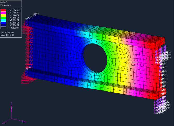
The primary results in a finite element analysis are grid point displacements and rotations. Element results such as stresses, strains, and strain energy density are derived from those results. Other results include element forces, MPC forces, SPC forces, and grid point forces.

Results of a finite element analysis are post-processed using a graphical tool.

The definitions of the output options can be found in the I/O Options Section. An overview of the result files can be found in the Results Output by OptiStruct section.

Information on stress, strain and force definitions regarding their coordinate system definition can be found in the section Element Results Representation in OptiStruct and on the respective element definitions.

Displacements

Displacements and rotations are computed in linear static, and frequency response analyses. In addition, in frequency response velocities and acceleration are computed.

Eigenvectors are the primary result in a normal modes and buckling analyses. In a normal modes analysis, they are normalized with respect to the mass matrix or with respect to the maximum vector component. In a buckling analysis, the latter always applies.

Displacements, velocities, accelerations, and eigenvectors are grid point results. They are plotted as a deformed structure, or as a contour on the undeformed structure. Some post-processors, such as Altair HyperMesh and Altair HyperView, also allow the animation of the displacements.

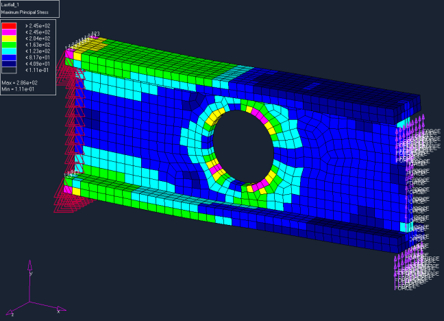
Deformed displacement contour plot

Stresses

The stresses are secondary results in a static analysis.

Stresses near notches and other sharp corners, point loads and boundary conditions, and rigid elements are often unreliable due to the singularities in these points. This is not a trait unique to OptiStruct, but is inherent in the finite element method itself. A mesh refinement in such places can improve the stress prediction. A theoretically infinite stress cannot be predicted by finite elements.

Stresses are primarily calculated at the Gauss integration points. These give the most accurate prediction. However, element stresses, corner stresses, and grid point stresses are provided.

Element stresses are calculated at the centroid of the element. They should only be post-processed using an assign plot. Contouring of element stresses vastly underestimates the extreme values due to the smearing across element boundaries.

The stresses of interest are usually found on the surface of a structure. Mesh refinement will actually not just improve the stress prediction but also change the location of the point of stress evaluation. Therefore, it is common practice to use a skin of thin membrane elements in 3D modeling, or rod elements in 2D modeling, to evaluate the stresses on element surfaces or edges, respectively. This method is accurate since it considers the correct condition of a stress-free boundary if no load is applied to the boundary. The method of skinning a model also has the advantage of much faster post-processing of solid models because only the membrane skin needs to be displayed.

Besides assign plots, elements stresses can be viewed in tensor plots that can help in the evaluation of the load path in a structure by evaluating the principal stress directions.

Corner stresses are computed by extrapolating the stresses from the Gauss points to the element grid points. Corner stresses are plotted in a contour plot. Corner stresses for solid elements are not available for normal modes analysis.

Grid point stresses are computed by averaging the corner stresses contributions of the elements meeting in a grid point. The averaging does not consider the condition of a stress-free boundary. Further, interfaces between different materials, where a stress jump normally can be observed, are not considered correctly because of the smearing of the stress. Grid point stresses are plotted in a contour plot.

For first order elements, grid point stresses do not provide higher accuracy over element stresses. For second order elements, the stress prediction might improve by using grid point stress over element stresses, considering the weaknesses mentioned above.

Assign plot of maximum principal element stress

Strains

Strains are secondary results.

They are calculated as elements strains. Remarks made above on element stresses apply here too.

Strain Energy Densities

Strain energy densities are secondary results in static and normal modes analysis.

They are calculated as element strain energy densities. Remarks made above on element stresses apply here too.

Forces

Element forces, MPC forces, SPC forces, and grid point forces are printed as tabulated output.

The default method of calculating stresses in OptiStruct produces values of stress components at the centroids of elements. (Typically a post-processor, such as HyperView, will then average these values to produce smooth contour plots). This method, while useful for viewing stress distribution, may underestimate stress maxima, especially on the surface of the body.

To provide higher accuracy stresses, OptiStruct supports grid point stress calculation. Grid point stresses are computed using the following steps:

The above approach produces continuous stress field, typically in the entire domain. Since, however, stresses can be discontinuous between different materials, OptiStruct supports calculation of separate grid point stress field per each material sub domain. The presence of more than one material is detected automatically and then grid point stresses are calculated for the entire domain and as a separate field for each material region.

Grid point stress calculation is activated through the I/O subcase command GPSTRESS. When activated, grid point stresses are produced in addition to default stress results – they can be found in a separate results subcase.

The present support for grid point stress capability has the following scope:

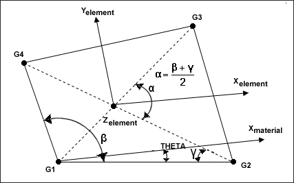
Elemental results (namely stresses, strains, element forces, flux and gradients) may be provided with reference to either the material system or the elemental system. For the HM, PUNCH, and OPTI output formats, results are provided with reference to the material system; for first order shell element results, PARAM, OMID may be used to output with either representation. The H3D and OUTPUT2 output formats, to which these elemental results are written as tensors, always contain results with reference to the elemental systems (unaffected by PARAM, OMID).

Since OptiStruct 10.0 optimization responses always match with the results written to the HM, PUNCH and OPTI formats and first order shell responses are consistent with the PARAM, OMID setting.

First Order Shell Elements

For first order shell elements (CQUAD4 and CTRIA3), the material system is defined as follows:

The elemental system is the bi-sector system for CQUAD4 elements (see figure) and the G1-G2 system for CTRIA3 elements.

Bi-sector coordinate system

For the H3D and OUTPUT2 formats this representation allows HyperView to perform coordinate system transformations on stress and strain tensors.

Second Order Shell Elements

The results for second order shells (CQUAD8 and CTRIA6), including shell strains, stresses and forces, are always presented in the local material coordinate system, as described in the manual for CQUAD8 and CTRIA6 elements.

Composite Shells

Shell-type strains and stresses for composite shells use the same representation as homogeneous shells. By shell-type results, strains and stresses calculated at Z1, Z2 using homogenized shell properties. Strains and stresses for individual plies are always presented in the respective ply coordinate system.

Solid Elements

For solid elements (CHEXA, CTETRA, CPENTA and CPYRA), the results are always provided in the material coordinate system.

Gap Elements

For gap elements, gap forces are represented in the gap coordinate system, as described on respective gap element manual pages (CGAP and CGAPG). Compression is positive.

OptiStruct allows Normal Modes Analysis results to be retrieved for use in Frequency Response Analysis or Transient Response Analysis using the modal method. Thus, multiple dynamic loading analyses can be performed using the eigenvalue results of a single normal modes analysis.

The following input I/O options and subcase information section entries may be used for this purpose:

EIGVSAVE is a subcase information entry that, if used within a normal modes analysis subcase, causes the eigenvalues and eigenvectors of that subcase to be written to an external data file. The external data file will use the default output file prefix unless the EIGVNAME I/O option is present, followed by an underscore, then followed by the EIGVSAVE integer argument and the .eigv extension.

For example, the input will save the eigenvector and eigenvalue results from a normal modes analysis to the file "test_file_50.eigv."

EIGVNAME = test_file

$

Subcase 10

Retrieving Eigenvalues and Eigenvectors for a Modal Frequency Response Analysis or for a Modal Transient Analysis

EIGVRETRIEVE is a subcase information entry that, if used within a modal frequency response analysis or a modal transient response analysis subcase, retrieves eigenvalues and eigenvectors from external data files. EIGVRETRIEVE may have multiple integer arguments, each referring to a different external data file. The external data files must have the default output file prefix unless EIGVNAME I/O option is present, followed by an underscore, followed then by the EIGVRETRIEVE integer argument and the extension .eigv.

For example, the following input can be used in a frequency response analysis subcase using the modal method to retrieve the eigenvalues and eigenvectors that were saved in the example above:

EIGVNAME = test_file

$

Subcase 40

Combining Eigenvalues and Eigenvectors from Two or More Normal Modes Analyses for a Single Modal Frequency Response or Modal Transient Response Analysis

The results of two or more normal modes analyses can be retrieved in combination for a modal frequency response analysis.

For example, a normal modes analysis is performed with the real eigenvalue extraction (EIGRL) data:

The results are written to an external data file as follows:

EIGVNAME = test_file

$

Subcase 10

In this case, all of the eigenmodes up to 50 Hz have been calculated and written to the file "test_file_50.eigv."

In order to perform a modal frequency response analysis with all of the modes up to 70 Hz, another normal modes analysis can be performed with the real eigenvalue extraction data:

This time, the results are written to an external data file as follows:

EIGVNAME = test_file

$

subcase 10

All eigenmodes between 50 Hz and 70 Hz are written to the file "test_file_70.eigv."

You can now run a modal transient response analysis with:

EIGVNAME = test_file

$

subcase 40

The real eigenvalue extraction data referenced in the modal transient response analysis subcase must not request eigenvalue and eigenvector results outside of the range of retrieved values. If it does, OptiStruct will terminate with an error. In this example, the following EIGRL cards are valid:

The following EIGRL cards would cause error terminations for this example:

It is recommended to use a frequency range without the maximum number of modes on the EIGRL bulk data entries referenced in normal modes analyses from which eigenvalue results are saved. If the maximum number of modes is specified and these eigenvalue results are retrieved by a modal frequency response analysis, and it cannot be determined whether all of the modes are obtained for the requested range, OptiStruct will terminate with an error.

For example, assume there are exactly 300 modes in the frequency range 0.0 to 5.0.0 Hz. Now assume that a normal modes analysis is performed referencing the EIGRL bulk data entry.

The eigenvectors and eigenvalues are saved as follows:

EIGVNAME = test_file

$

Subcase 10

All 300 modes in the range of 0 to 50.0 Hz are extracted and saved to the file "test_file_50.eigv."

Now try to retrieve these results to use in a modal frequency response analysis, as follows:

EIGVNAME = test_file

$

subcase 40

EIGVRETRIEVE = 50

where the referenced EIGRL definition is:

This will cause an error termination because it is known (through the external data file) that there are 300 modes within the 0.0 to 50.0 Hz range, but do not know if this is all of the modes.

If the EIGRL definition referenced in the normal modes analysis were specified as:

and only 300 modes were found, you would know that these are all of the modes within the 0.0 to 50.0 Hz range, and would retrieve the saved eigenvalue results in this case. OptiStruct would not terminate with an error.