The Contour panel allows you to create contour plots of a model and graphically visualize the analysis results.
To access the Contour panel, click on the Contour button  on the Results toolbar, or select Plot > Contour from the Results menu.
Panel Usage
The options in the panel will vary, depending on the type of model and results files that are loaded:
| • | Set the display options for the contour plot which is automatically applied to the model. |
When you are finished making all your selections, create a contour plot by clicking Apply in the lower middle section of the panel.
After a contour is applied, you can click Cache to add this result to an internal cache. This can be used to cache all of the results that are likely to be viewed multiple times in a given session, thereby avoiding re-computation and allowing you faster switching between scalar results. See the Caching Results topic for additional information.

Contour panel
Panel Options
This section allows you to select the result data type and the corresponding data component type that should be used to calculate contours.
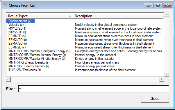
Use the first drop-down menu under Result type to select one of the available result types. The options change depending on the currently loaded result file. Each result type is followed by a letter that indicates the category to which it belongs. (t) indicates a tensor-type result, such as stress or strain tensors. (v) indicates a vector-type result, such as displacement, velocity, and acceleration. (s) indicates a scalar-type result. (c) indicates complex results. The expansion button,  , opens the Choose From List dialog where you can filter result types for quick selection. , opens the Choose From List dialog where you can filter result types for quick selection.
The second drop-down menu in the Result type section allows you to choose the data component type. The list of available components is based on the selected result type. For example:
|
Result type
|
Component options
|
Displacement (v)
|
Mag, X, Y, or Z
|
Stress (t)
|
vonMises, Signed vonMises, Tresca, Triaxiality, Lode Param xi, Lode Param theta, P1(major), P2(mid), P3(minor), In-plane P1(major), In-plane P2(minor), MaxShear, Intensity, Pressure, , XX, YY, ZZ, XY, YZ, or ZX
|
1D stress
|
Multiple options are listed for various elements such as: CELAS, CROD, CBAR, CBEAM, etc.
|
Energy (s)
|
No component selection is necessary.
|
Return to Panel Usage section
|
Allows you to display a contour for a specified element layer when a layer definition is available for an element. The contour will be applied to all layers defined in the model. If an element has no layer definition, as in a mass or solid, the contour is also displayed regardless of which layer is selected.
The options that control how layers will be displayed are:
|
Max
|
Displays the maximum value among the layers for each entity.
|
Min
|
Displays the minimum value among the layers for each entity.
|
Extreme
|
Displays the maximum absolute values among the layers for each entity.
|
Sum
|
Displays the (scalar) sum of all values among the layers for each entity.
|
Average
|
Displays the (scalar) average value among the layers which contain data for each entity.
Layers that do not have values (N/A result) will not contribute to the averages (see the example below):
Layer 1 - 10.0
Layer 2 - 26.0
Layer 3 - 30.0
Average is (10+26+30)/3 = 66/3 = 22.0
However if:
Layer 1 - 10.0
Layer 2 - 26.0
Layer 3 - N/A
Average is (10+26)/2 = 36/2 = 18.0
|
Range
|
Displays the difference between the maximum and minimum values among the layers for each entity.
The range is shown as zero if there is only one value (for example, for solid elements that do not have any layers or section points reported).
|
Count
|
Displays a count of the layers for the given data type. By default, the total number of layers/plies are given for each node/element. When used with a Layer Filter or Value Filter, the Count aggregation mode will have slightly different behavior (based on the filter criteria).
|
MaxLayer
|
Identifies and plots the layer by name that contributes to the maximum value for each entity.
|
MinLayer
|
Identifies and plots the layer by name that contributes to the minimum value for each entity.
|
ExtremeLayer
|
Identifies and plots the layer by name that contributes to the extreme (absolute maximum) value for each entity.
|
Top/Bottom
|
Displays the contour of top and bottom layers in the same plot. You can use this option to specify which layer should be on the top or bottom.
Click the Top/Bottom layer setting icon  to display the Top/Bottom Layer dialog: to display the Top/Bottom Layer dialog:
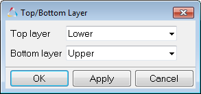
Use the drop-down menu to specify a location (Lower, Mid, or Upper) for the Top layer and Bottom layer.
| - | Click OK to apply the settings/changes and exit the dialog. |
| - | Click Apply to apply the settings/changes to the contour plot. |
| - | Click Cancel to disregard the settings/changes and exit the dialog. |
|
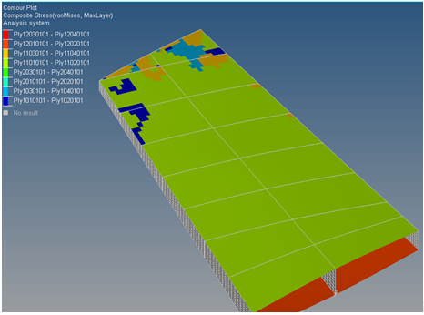
MaxLayer Contour Plot - Example
Note (for Layers): The maximum, minimum, or extreme value can be queried using Quick Query, Query Panel, Measures, or from the Notes entry fields (in addition to the layer name). A Category Legend appears for each of these contour plots.
Only in the case of results based at the elemental centroid, would one layer per element be displayed. For corner bound or nodal bound results (in the case of averaging), different layers may contribute to the max/min/extreme value at each corner/node of the same element.
Click here to view a table in the Derived Load Steps topic which explains the behavior of layer aggregation (Min/Max/Range) in combination with the Min/Max/Range Envelope loadstep types.
|
Solver specific layer options
|
Solver dependent label(s). For example, Z1 and Z2 indicates the upper and lower shells layers in a Nastran model.
For example:
Element 1 Lower = -20, Upper = 10
Element 2 Lower = -5, Upper = 30
Lower layer:
Legend Max = -5, Min = -20
Upper layer:
Legend Max = 30, Min = 10
Min layer:
Legend Max = -5, Min = -20
Max layer:
Legend Max = 30, Min = 10
Extreme layer:
Legend Max = 30, Min = -20
|
Layer Filter 
|
Allows you to reduce the layer list available for aggregation for the data types which have layers (for example, plies in composite stress/strains or any vector result with layers).
|
Use corner data
|
If corner data is available, the Use corner data option is enabled. If you activate the option, HyperView displays color bands by interpolating available corner results within each element. A discontinuity of the result distribution across element boundaries can be seen.
|
Return to Panel Usage section
|
Before creating a contour plot, you may pick one or more entities from the model. You can do this by picking entities directly from the screen, using the quick window selection, or clicking the Elements, Components, or Assemblies input collector and using the extended entity selection menu. If no selection is made, the contour will be applied to displayed elements, components, or assemblies by default. See Selecting Entities Using the Input Collector for more information on selecting entities. For contour or multiple models see MultiModel Result Plotting for additional information.
Note: For MBD models, Systems (or Markers) can also be selected. Selection will be available if the results file has any type of results that are bound to Systems/Markers (for example; forces or moments).
|
Return to Panel Usage section
|
This drop-down menu allows you to select the result coordinate system to be used to contour the results. The available options are dependent on the current selection for Averaging method. You can select the analysis, element, or global coordinate system as well as a user-defined system. The System input collector is enabled when User System is selected.
|
Global System
|
Transforms to the global system.
(proj: none) indicates that no projection rule is selected for shells. When a projection rule is selected (using the Projection Rule… button) it is displayed, for example, (proj: y, x).
|
Elemental System
|
Transforms results to the element coordinate system. In HyperView, the element coordinate system is defined by element connectivity.
|
Material System
|
Transforms to the material system.
This option is only available when the Advanced Result Math template is selected in the Load Model panel and a solver input deck is loaded.
Note: For plotting data types that do not have relevance to the Material system (for example, Stress with a Z1 and a Z2 data type), it is not advised that you apply the Resolved-In system of Material, because this may result in incorrect transformations.
|
Ply System
|
Transforms to the ply system.
This option is only available when the Advanced Result Math template is selected in the Load Model panel and a solver input deck is loaded.
Note: For plotting data types that do not have relevance to the Ply system (for example, Stress with a Z1 and a Z2 data type), it is not advised that you apply the Resolved-In system of Ply, because this may result in incorrect transformations.
|
Analysis System
|
Displays the vector and tensor results as they are output from the solver.
|
User System
|
This option is available when the results file contains a user-defined coordinate system. Click the System input collector to select a system by ID or pick from the screen. Markers can also be selected for MBD models.
(proj: none) indicates that no projection rule is selected for shells. When a projection rule is selected (using the Projection Rule… button) it is displayed, for example, (proj: y, x).
|
Use tracking system
|
If a tracking system has been activated in the Tracking panel, the Use tracking system option is enabled. If you activate this option, the results will be transformed and resolved in the activated tracking system.
This option is not available if you are using the Modal or Linear Static animation mode.
|
Return to Panel Usage section
|
This option (introduced in version 14.0.130) primarily controls what HyperView will do when the solver results file does not contain results for mid-side nodes on 2nd order elements.
If the check box is turned ON, HyperView will show mid-side node results. Refer to the Mid-side Node Elemental Results in Contour topic for details on how the calculation is performed if the solver does not output results on mid-side nodes. If the check box is OFF, HyperView will not show any results on the midside nodes.
This option is disabled whenever any of the following conditions are met:
| • | Loaded results do not have 2nd order elements. |
| • | Results are on nodes, components, or systems. |
| • | Averaging mode is set to Max/Min/Extreme of corner. |
| • | Use corner data option is off and the averaging mode is set to None. |
Return to Panel Usage section
|
This drop-down menu allows you to choose the averaging method:
None
|
No averaging method is used. Color will be displayed in element-based results, a solid color for centroidal results, or multiple color bands within an element.
|
Simple
|
Tensor and vector components are extracted and the invariants are computed prior to averaging.
|
Maximum
|
Extracts the maximum values from the surrounding elements attached to a node. The tensor and vector components are extracted and the invariants are computed for each element (or corner) prior to averaging to a node. For results components, the corresponding components from each element corner (or centroid) are extracted and then the maximum value is assigned to the shared node. For invariants, the corresponding invariants are calculated from each tensor at the element corners and then the maximum value is assigned to the node.
For example, as shown in Nodal Averaging of Elemental Results, there are four tensors, [A2], [B1], [C3], and [D4] at four corners at Node 400.
The maximum average of the xx component at Node 400 is:

|
Minimum
|
Extracts the minimum values from the surrounding elements attached to a node. The tensor and vector components are extracted and the invariants are computed for each element (or corner) prior to averaging to a node. For results components, the corresponding components from each element corner (or centroid) are extracted and then the minimum value is assigned to the shared node. For invariants, the corresponding invariants are calculated from each tensor at the element corners and then the minimum value is assigned to the node.
For example, as shown in Nodal Averaging of Elemental Results, there are four tensors, [A2], [B1], [C3], and [D4] at four corners at Node 400.
The minimum average of the xx component at Node 400 is:

|
Advanced
|
Tensor or vector results are transformed into a consistent system and then each component is averaged separately to obtain an average tensor or vector. The invariants are calculated from this averaged tensor or vector.
|
Difference
|
The difference between the maximum and minimum corner results at a node.
|
Max of corner
|
Extracts the maximum value from all the corners of an element and the value is shown at the centroid of the element. The tensor and vector components are extracted and the invariants are computed for each corner prior to assigning to the element centroid. For result components, the corresponding components from each corner is extracted and then the maximum value is assigned to the element centroid. For invariants, the corresponding invariants are calculated from each tensor at the element corners and then the maximum value is assigned at the centroid.
For example, as shown in Nodal Averaging of Elemental Results, there are four tensors at each corner of the element A: [A1], [A2], [A3], and [A4].
The max of corner aggregation of the xx component at the Element A centroid is:

This averaging option is only available when the Use corner data option is checked. The Variation option is automatically disabled for this averaging method.
|
Min of corner
|
Extracts the minimum value from all the corners of an element and the value is shown at the centroid of the element. The tensor and vector components are extracted and the invariants are computed for each corner prior to assigning to the element centroid. For result components, the corresponding components from each corner is extracted and then the minimum value is assigned to the element centroid. For invariants, the corresponding invariants are calculated from each tensor at the element corners and then the minimum value is assigned at the centroid.
For example, as shown in Nodal Averaging of Elemental Results, there are four tensors at each corner of the element A: [A1], [A2], [A3], and [A4].
The min of corner aggregation of the xx component at the Element A centroid is:

This averaging option is only available when the Use corner data option is checked. The Variation option is automatically disabled for this averaging method.
|
Extreme of corner
|
Extracts the extreme value from all the corners of an element and the value is shown at the centroid of the element. The tensor and vector components are extracted and the invariants are computed for each corner prior to assigning to the element centroid. For result components, the corresponding components from each corner is extracted and then the extreme value is assigned to the element centroid. For invariants, the corresponding invariants are calculated from each tensor at the element corners and then the extreme value is assigned at the centroid.
For example, as shown in Nodal Averaging of Elemental Results, there are four tensors at each corner of the element A: [A1], [A2], [A3], and [A4].
The extreme of corner aggregation of the xx component at Element A centroid is:

This averaging option is only available when the Use corner data option is checked. The Variation option is automatically disabled for this averaging method.
|
Variation (%)
|
The relative difference at a node from corresponding corner values with respect to the value range from all nodes in the selected components.
If the variation in the results is smaller than the specified percentage, HyperView will average the corner results to the nodes. If the variation is larger than the specified percentage, HyperView will keep the discontinuity of the results.
This option is not available for all averaging methods.
|
Return to Panel Usage section
|
The averaging options allow you to limit the averaging of results to only a group of elements that are considered to be bound by same feature angle or face.
Typically averaging is performed for all connected elements in a part without any regard for adjacent elements that are modeled around sharp edges or T-connections.
Click Averaging Options (located in the middle of the panel) to display the Averaging Options dialog.
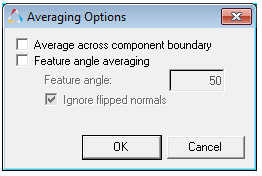
Note: Feature angle averaging is only applicable when the Simple or Advanced averaging methods are used, and no Variation is selected. As the nodes shared by elements that do not meet the feature angle criteria can have different values on either side of the feature angle, the output is always presented as corner bound values on each element.
Average across component boundary
|
Enables the nodal averaging across the component boundary. The contribution for a shared node will come from every component associated with that node, while all of the other averaging principles remain.
|
Feature angle averaging
|
Activate this option to specify the threshold value for elements to be considered as part of the same feature by specifying a Feature angle value. All of the adjacent elements whose normals are less than or equal to the threshold value are averaged.
The output of this contour is always corner based data (no centroid values). A feature angle average calculation example is shown below:
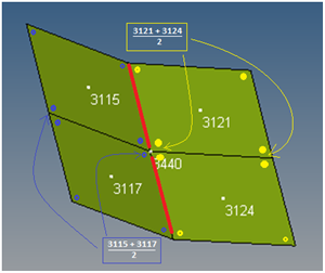
Result at common node 3440:
| • | E 3115, average of corner nodes for element 3115 and 3117 |
| • | E 3121, average of corner nodes for element 3121 and 3124 |
| • | E 3117, average of corner nodes for element 3115 and 3117 |
| • | E 3124, average of corner nodes for element 3121 and 3124 |
|
Feature angle
|
Allows you to specify the value to be used in the Feature angle averaging calculations. The default is 30 degrees. All of the elements whose normals are less or equal to the specified threshold value are averaged. The value can range from 0 to 180 degrees.
For element feature angle calculation, the current model position is used. Only shell elements feature angles are considered, therefore all solid and beam elements will be included in the averaging calculation (see the example below):
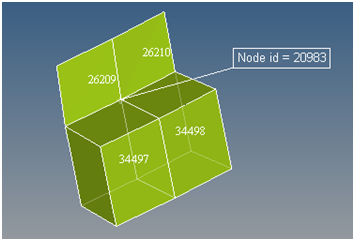
The result at common node 20983 = the average of corner nodes for all four elements.
|
Ignore flipped normals
|
This option is checked by default (for feature based averaging) to allow for any modeling discrepancies to be disregarded.
Consider the picture and description below which shows two adjacent elements whose normals are flipped as a consequence of a model setup discrepancy:
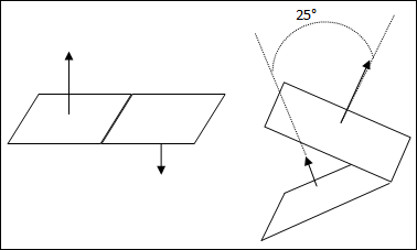
In the example above, the feature angle threshold for averaging is set at 30 degrees. The image on the left side has an angle between adjacent element normals close to 180 degrees and therefore does not meet the criteria of the 30 degree threshold. The image on the right has the angle between normals less than 30 degrees, and the threshold criteria for feature angle is satisfied. However, this could be a modeling discrepancy that should be accounted for, perhaps allowing the averaging of values for elements on the left image, but not allowing averaging of elements on the right image. This can be accomplished by activating the Ignore flipped normals option.
If strict adherence to the angle between adjacent element normals is to be enforced, then uncheck this option.
See the examples provided below:
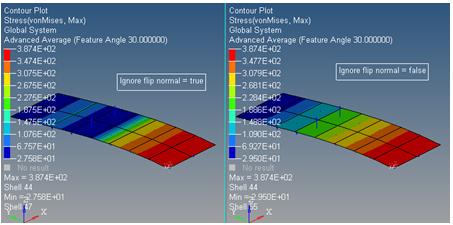
|
Note - The Legend will automatically update and reflect that feature angle averaging is activated.
Return to Panel Usage section
|
Activating the Envelope trace plot option allows you to track the results from Envelope subcases or simulations.
|
None
|
No Envelope subcases or simulations are tracked.
|
Subcase
|
Tracks the results from an Envelope subcase.
|
Simulation
|
Tracks the results from an Envelope simulation.
|
Note - For the envelope trace plot (subcase or simulation), a Category Legend is shown with subcases or simulations. You can choose to see the IDs or the labels of the subcases/simulations by checking or unchecking the Show Category ID option in the Edit Legend dialog. The Envelope Trace Plot option will be disabled if Range is selected for an Envelope subcase/simulation.
|
Return to Panel Usage section
|
The value filter options allow you to specify threshold criteria for processing results only in a specific range.
Mode
|
Select one of the following options from the drop-down menu:
None (*Default setting)
<= (less than or equal to)
>= (greater than or equal to)
Range
|
Value
|
Use the field(s) to specify a numerical value or range of values.
|
Any entities having values outside of filter parameters will be displayed as gray in the graphics area.
See the Value Filter topic for additional information.
Return to Panel Usage section
|
The display options change the appearance of the contour colors and are automatically applied to the model as you enter information.
Discrete color
|
Produces discrete color bands on contour plots with distinct boundaries between contour levels. This option uses a texture mapping capability in your graphics card. If your graphics card does not support texture mapping, the performance may slow down.
|
Interpolate
colors
|
Interpolates the contour colors from the undeformed shape (with a zero value) to the result variable reported from the solver. If you do not select Interpolate colors, the contour colors remain the same for all frames. This is only applied to modal and linear static animation.
|
Return to Panel Usage section
|
Max
|
Enter the value to be assigned to the highest color in the contour plot. Activate the Max check box to apply the value.
The new value is also changed in the Values section of the Edit Legend dialog.
If a value entered for threshold Max is invalid, it will not be applied and the panel will be updated to reflect the actual state.
|
Min
|
Enter the value to be assigned to the lowest color in the contour plot. Activate the Min check box to apply the value.
The new value is also changed in the Values section of the Edit Legend dialog.
If a value entered for threshold Min is invalid, it will not be applied and the panel will be updated to reflect the actual state.
|
Multiplier
|
Enter the multiplier for scaling all the result values. An additional line will be added to the legend if a multiplier value is entered.
|
Offset
|
The offset value affects the contour value, contour min/max, and the legend min/max. An additional line will be added to the legend if an offset value is entered.
The offset value option can be useful for:
| • | converting temperatures from Kelvin to Celsius |
| • | converting temperatures from Kelvin to Fahrenheit
(by using the offset and multiplier options) |
| • | calculating factor of safety as (1 – stress/allowableStress) etc. |
Note: The multiplier takes effect first, therefore you can perform operations like y=mx + C on the contour (where m is the multiplier and C is the offset).
|
Edit Legend
|
Opens the Edit Legend dialog where you can change the legend properties.
|
Return to Panel Usage section
|
The following options allow you to manage the result display.
|
Overlay result
display
|
Overlays contour, tensor, and vector results in the same window. If all results are displayed simultaneously, available memory may be affected.
|
Clear Contour
|
Clears the contour and returns the model to its original state.
|
Create Plot Style
|
Opens the Create/Update Contour Plot Style dialog, which allows you to create or update a result plot style based on the current settings of the contour.
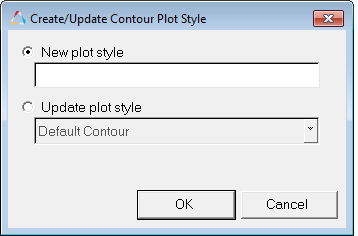
A contour plot needs to be current in order to create a new style or modify an existing one. All the settings of the contour plot (corner data options, averaging, resolved in systems, default data type/components, display options, legend, etc.) are captured in the named style.
|
Show/Clear
Iso Value
|
Displays/clears iso values.
|
Projection Rule
|
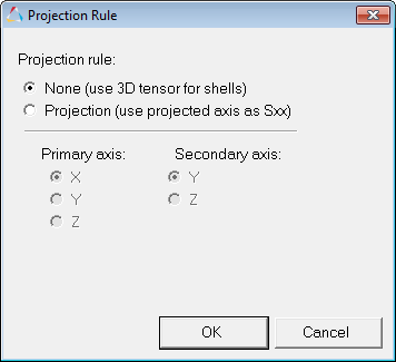
This button (located on the far right side of the panel) opens the Projection Rule dialog where you can select the primary and secondary axes from either the global or user-defined system (selected for Resolved in). When the primary axis is perpendicular to the shell plane, the secondary axis is used.
|
Query Results
|
Opens the Query panel where you can view and export properties and other information related to nodes, elements, components, and systems contained in the active model.
|
Return to Panel Usage section
|
Contour Plots
A contour plot generates color bands on the model, based on the values found in the results file.
HyperView processes these values as described below:
Nodal results such as temperature, displacement, velocity or acceleration are stored at the nodes. Colors are displayed at the nodes using nodal values directly or transformed values using the system selected for Resolved in.
|
The values can be located at the element centroidal or corners. The Use corner data option is available when a result file contains corner results. You can display the results at the elements directly without using an averaging method, or average them to nodes using the simple or advanced averaging method. The calculated values shown in the legend may vary due to the different averaging methods.
Centroidal results
|
A solid color is displayed at the elements using the elemental centroidal results directly.
|
Corner results
|
The values are located at the corners of an element. Discontinuous color bands are displayed within each element using corner results.
|
None
|
When no averaging method is used, the results remain as element binding, so you can query results using the Elements option in the Query panel or Measure panel.
|
|
HyperView averages the results to the nodes based on a user-specified variation percentage. If the Variation (%) option is not used, HyperView simply averages the elemental values to nodes and the calculated results can be queried at nodes. If Variation (%) is enabled, HyperView averages elemental values to the nodes at the areas where the variation is less than the specified percentage and leaves other areas as they are without averaging. In this case, HyperView represents results in element binding, so you can query results using the Elements input collector on the Query panel. When entering the Query panel, you can see the contour values are displayed as available elemental items. See the Variation Percentage Control for further explanation.
|
Advanced averaging is similar to simple averaging. Without using variation, HyperView averages elemental values to all nodes. The calculated nodal results can be queried using the Nodes input collector on the Query panel. When using variation, the results remain as element bound and are queried using the Elements input collector.
|
HyperView calculates the difference of corner or centroidal results and assigns it to a node. You can query results using the Nodes input collector on the Query panel.
|
| • | The Complex filter options allow you to extract one of the components from a complex number such as mag, phase, real, or imaginary separately. |
| • | HyperView automatically recognizes a subcase with complex results and loads the model and results in the modal mode. |
| • | Complex filter is activated when a complex result type is selected. It is only applied to result types that are provided directly from solvers such as Displacements X, Y, Z or Stress Sxx, Syy, Szz, etc. This filter is not applicable to derived results such as Displacement magnitude or vonMises. |
| • | If you measure contour nodal results as a complex number using mag cos(wt-phase), a sinusoidal (Cosine) curve with phase shift is calculated. |
| • | If you measure any of the components of a complex number (mag, phase, real or imaginary), the curve is shown as constant. |
|
HyperView will use the Mag across all the frequencies. This will be useful to examine the peak across all the frequencies. Essentially, the curve created from measure should agree with the curve of magnitude you get from the PCH file in the complex plot.
|
An Envelope loadstep (with Min, Max, Extreme, and Range options) is a single simulation step containing results from multiple simulation steps for the model. Result transformations and Averaging options are not available for data contoured from an Envelope loadstep. All results are presented in the Analysis system with no averaging.
|
Supported Results for 1D Elements
HyperView supports 1D (or line) element results. Each 1D element has two corners and a base (centroid) location for elemental results. HyperView supports contour colors for the base (centroid) location only. This means an element will have only one color when the Use corner data option in the Contour panel is not selected. When the Use corner data option is selected, the element contour color becomes gray. However, you can still use the Query panel to query corner results.
For HyperMesh Users
If you are familiar with HyperMesh, you know that it contains a contour panel as well. The Contour panel in HyperView processes result values differently and more accurately than the HyperMesh Contour panel. In the HyperMesh contour panel, the elemental results are averaged to nodes and the averaged values are used for the colors and legend display. By doing this, the Max/Min result values are averaged, thus lowering the Max values in the legend. This may cause some confusion for HyperMesh users when they use the Contour panel in HyperView. To match a HyperMesh contour plot in HyperView, verify that the Use corner data option is deactivated, select the Simple averaging method without variation, and use Analysis System for Resolved in. This is done because in HyperMesh, the results are always treated as scalars, so transformation to other systems cannot be applied. When the Analysis System option is used, the original values are extracted directly from the result file for averaging. Considering the extended support of transformation and averaging methods in HyperView, we recommend using HyperView for an accurate post-processing of results.
How Do I...
| 1. | From the Contour panel Result type drop-down menu, select the data type that should be used to calculate the contours. |
| 2. | Select a data component from the second drop-down menu below Result type. If you select Mag (Magnitude), the results system is disabled since magnitude is the same for any coordinate system. |
| 3. | For Selection, pick one or more entities from the model. |
| 4. | For Resolved in, select the coordinate system that will be used to calculate the results. |
| - | If User System is selected, use the System input collector to select a system by ID. |
| 5. | Activate the relevant check boxes for Display options, Legend threshold, and Result display control. |
| 6. | Click Apply. The contour plot is displayed. |
|
| 1. | From the Contour panel Result type drop-down menu, select the data type that should be used to calculate the contours. |
| 2. | Select the data component from the second drop-down menu below Result type. |
| 3. | If the element has layers defined, select the relevant option for Entity with layers. |
| 4. | If corner data is available, activate Use corner data to display color bands by interpolating available corner results within each element. |
| 5. | For Selection, pick one or more entities from the model. |
| 6. | For Resolved in, select the coordinate system that will be used to calculate the results. |
| - | If User System is selected, use the System input collector to select a system by ID. |
| 7. | Select an averaging method. |
| 8. | For Use variation (%), enter a percentage for the variation range. |
| 9. | Activate the relevant check boxes for Display options, Legend threshold, and Result display control. |
| 10. | Click Apply. The contour plot is displayed. |
|
| 1. | From the Contour panel, click Edit Legend. The Edit Legend dialog is displayed. |
| 2. | Select the attributes that you want to apply to the legend. The changes are previewed on the sample legend, located on the right side of the dialog. |
|
See Also:
Edit Legend
Composites Post Processing
Layer Filter
Value Filter
Caching Results
Mid-side Node Elemental Results in Contour
Post-processing Stress Results Using the Contour Panel
List of Tcl/Tk poIContourCtrl Class Commands
Using Scalable Fonts under Linux to Render Text


![]() on the Results toolbar, or select Plot > Contour from the Results menu.
on the Results toolbar, or select Plot > Contour from the Results menu.