Zero-dimensional Elements

Elements in this group only connect to grid points having a single degree of freedom at each end. Elements also included in this group are those that connect to scalar points at one end and ground at the other, like the following:

One-dimensional Elements

Elements in this group are represented by a line connecting grid points at each end. The following actions involving forces (and displacements) at each end are possible:

The elements in this category are:

The properties for these elements are defined on PBEAM, PBAR, PBUSH, PBUSH1D, PGAP, PROD, and PWELD, respectively.

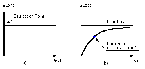
Two-dimensional Elements

Two-dimensional elements are used to model thin-shell behavior, which incorporates in-plane or membrane actions, plane strain, and bending action (including transverse shear characteristics and membrane-bending coupling actions). Reissner-Mindlin shell theory is used to model bending. A plane strain option is available for pure 2D applications. The element shapes may be triangular (CTRIA3) or quadrilateral (CQUAD4). Second order triangular (CTRIA6) and quadrilateral (CQUAD8) shell elements are also available. The shell properties, including the behavior, are defined on the PSHELL entry.

The first order shell element formulation for CQUAD4 and CTRIA3 has the special characteristic of using six degrees of freedom per grid. Hence, there is stiffness associated to each degree of freedom. In some finite element codes, shell elements do not have a drilling stiffness normal to the mid-plane, which may cause singular stiffness matrix. Then, a user-defined artificial stiffness value is assigned to this degree of freedom to avoid the singularity.

The second order shell elements (CTRIA6 and CQUAD8) have five degrees of freedom per grid. Rotational degrees of freedom without stiffness are removed through SPC.

Another form of two-dimensional elements may also be used to model thin buckled plates. These elements support shear stress in their interior and extensional forces between their adjacent grid points. These elements are used in situations where the bending stiffness and axial membrane stiffness of a plate is negligible. The elements are quadrilateral and are defined as CSHEAR. Their properties are defined on the PSHEAR entry.

Three-dimensional Elements

The three-dimensional solid elements are used to model thick plates, solid structures. In general, structures in which the lateral dimensions are of the same order of magnitude as the longitudinal dimensions can support the use of three-dimensional solid elements in modeling. The elements in this category are the CHEXA, CPENTA, CPYRA, and CTETRA elements. The property definition associated with these elements is called PSOLID.

Offset for One-dimensional and Two-dimensional Elements

Some one-dimensional and two-dimensional elements can use offset to “shift” the element stiffness relative to the location determined by the element’s nodes. For example, shell elements can be offset from the plane defined by element nodes by means of ZOFFS. In this case, all other information, such as material matrices or fiber locations for the calculation of stresses, are given relative to the offset reference plane. Similarly, the results, such as shell element forces, are output on the offset reference plane.

Offset is applied to all element matrices (stiffness, mass, and geometric stiffness), and to respective element loads (such as gravity). Hence, in principle, offset can be used in all types of analysis and optimization.

However, caution is advised when interpreting the results, especially in linear buckling analysis. Without offset, a typical simple structure will bifurcate and loose stability “instantly” at the critical load. With offset, though, the loss of stability is gradual and asymptotically reaches a limit load, as shown below in figure (b):

In practice, the structure with offset can reach excessive deformation before the limit load is reached. (Note that more complex structures, such as frames or structures experiencing bending moments, buckle via limit load even in absence of ZOFFS on the element card). Furthermore, in a fully nonlinear approach, additional instability points may be present on the limit load path.

Elements for Geometric Nonlinear Analysis

Special element formulations are available for geometric nonlinear analysis. As a general rule, property definitions that are only applicable in geometric nonlinear analysis are defined on extensions to the original property. The extensions are grouped with the base entry by sharing the same PID. In the case of a subcase that is not a geometric nonlinear analysis, these extensions are ignored. The following extensions are available: PSHELLX, PSOLIDX, PBARX, and PBEAMX. Property defaults can be set for shells (XSHLPRM) and solids (XSOLPRM) that may replace the use of property extensions. All other properties are used as they are.

Example:

PSHELL, 3, 7, 1.0, 7, , 7

PSHELLX, 3, 24, , , 5

Non-structural mass may be specified in two different ways.

When non-structural mass is defined in this way, it is considered in all analyses.

These non-structural mass definitions must be selected for use in an analysis through the NSM subcase information entry. Only one NSM subcase information entry can exist in a model and it must occur before the first SUBCASE statement.

The bulk data entry NSM and its alternate form NSM1 allow you to define a value of non-structural mass per unit area or non-structural mass per unit length to be applied to a selected list of elements.

The bulk data entry NSML and its alternate form NSML1 allow you to allocate and smear a lumped non-structural mass value to be evenly distributed over a list of elements. The non-structural mass value per unit area or per unit length to be applied to the elements is computed as:

Where, n is the number of elements in the set and M is the value of the lumped mass, Ai is the area of element i, and Li is the length of element i. The NSML and NSML1 entries cannot mix area and line elements on the same entry. The area elements are: CQUAD4, CQUAD8, CTRIA3, CTRIA6, and CSHEAR; line elements are: CBAR, CBEAM, CTUBE, CROD, and CONROD.

Combinations of NSM, NSM1, NSML, and NSML1 can be formed using the bulk data entry NSMADD.

An element can have more than one non-structural mass value specified for it. The actual non-structural mass value will be the sum of all of the individual non-structural mass values.

Virtual Fluid Mass mimics the mass effect of an incompressible inviscid fluid in contact with a structure. It does not represent the actual mass of the fluid. There is no mesh needed for the fluid domain. The Virtual Fluid Mass represents the full coupling between acceleration and pressure at the fluid-structure interface. A dense mass matrix is generated among damp grids at the fluid-structure interface. This simulation is applicable to automobile containers, such as a fuel tank, which hold non-pressurized fluids.

Assumptions

MFLUID Interface

If a fish can swim to every point inside fluid domain without leaving the fluid, the fluid domain can be represented by a single MFLUID card in the bulk data section. Each MFLUID card in the bulk section can only be referred to by a single MFLUID card in the control section. Multiple bulk data MFLUID cards can be referred by a single MFLUID card in the control section. Symmetry and anti-symmetry options can be applied to a MFLUID card.

If PARAM,VMOPT,1 is used (default), the virtual mass is included in the regular mass matrix and it can be applied to both direct and modal dynamic subcases. Because the virtual mass matrix is dense for the damp grids, the computational time increases significantly. However, you have the option to use PARAM,VMOPT,2; although, PARAM,VMOPT,2 can only be applied to modal dynamic subcases. In this case, the virtual mass is added after the eigen solution, and the computational time is not increased significantly. When PARAM,VMOPT,2 is used, the dry modes are computed without adding virtual mass in the computation. Then the modes are modified based on the virtual mass matrix.

Theory

The elemental pressure and acceleration are calculated with respect to the source potential of the element. The pressure is calculated based on displacement potential as:

If the source potential of element j is , the pressure can be represented as:

An additional area integration is done to convert pressure into force.

Similarly, the acceleration vector can be represented as:

Using the force and acceleration, the effective mass matrix can be calculated.

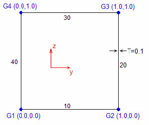
In addition to using predefined beam cross-sections selected by the TYPE field on the PBARL and PBEAML bulk data entries, defining arbitrary beam cross-sections. This is referred to here as section definitions. To define an Arbitrary Beam Section, HYPRBEAM should be entered into the GROUP field on the PBARL and PBEAML bulk data entries. Also, the ND field should specify the number of dimensions input during the definition of the arbitrary beam section in the DIMi fields of the PBARL and PBEAML bulk data entries.

Section definitions are contained within the bulk data section of the input file. A section definition begins with the statement BEGIN and ends with the statement END. Section definitions are referenced from a PBARL or PBEAML definition through the NAME field. The NAME entered on the PBARL or PBEAML definition must match the NAME following the BEGIN statement.

The section is defined by a 2D finite element mesh. The finite element mesh is composed of nodes (specified by GRIDS entries), which are connected by 2-node, 3-node, 4-node, 6-node or 8-node elements (specified by CSEC2, CSEC3, CSEC4, CSEC6, or CSEC8 entries, respectively). These elements reference PSEC entries; these provide a material reference for all elements and thickness information for the 2-noded CSEC2 elements.

The following is an example of a simple thin-walled section definition named SQUARE:

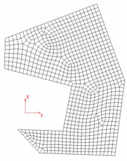
The following is an example of a solid section definition named CUTOUT:

Rigid elements and multi-point constraints are used to constrain one or more degrees of freedom to be equal to linear combinations of the values of other degrees of freedom.

Rigid elements are equations generated internally. You provide the connection data only. Rigid elements function as rigid bodies; therefore they are also known as rigid bodies or constraint elements. Internally, they are treated the same way as multi-point constraints.

The RROD element can be used to model a pin-ended rod which is rigid in extension. One equation of constraint will be generated for this element. The RBAR element can be used to model a rigid bar with six degrees of freedom at each end. Anywhere from one to six (depending on your input) equations of constraint will be generated for this element.

The RBE1 and RBE2 elements are rigid bodies connected to an arbitrary number of grid points. The number of equations of constraint generated is equal to or greater than one, depending on the dependent degrees of freedom selected by you. For the RBE1 element, the independent degrees of freedom are six components of motion that must be jointly capable of representing any general rigid body motion of the element; whereas for the RBE2 element, the independent degrees of freedom are the six components of motion at a single grid point.

The RBE3 element provides for specification from one to six equations of constraint developed from the relation that the motion at a "reference grid point" is the least square weighted average of the motion at other grid points. This element is generally used to "beam" loads and masses from a reference point to a set of grid points. Multi-point constraints are equations in which you explicitly provide the coefficients of the equations. Each multi-point constraint is described by a single equation that specifies a linear relationship for two or more degrees of freedom. Multiple sets of multi-point constraints can be provided in the bulk data section. In the subcase information section, the multi-point constraints are assigned to the specific load case using the MPC statement.

The bulk data entry MPC is the statement for defining multi-point constraints. The first coordinate mentioned on the card is taken as the dependent degree of freedom (that is, the degree of freedom that is removed from the equations of motion). Dependent degrees of freedom may appear as independent terms in other equations of the set; however, they may appear as dependent terms in only a single equation.

Some uses of multi-point constraints are:

When using rigid elements or multi-point constraints, you must make sure that the following requirements are satisfied:

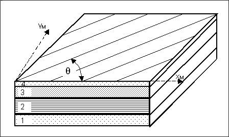
Overview

Plates and shells can be made of layered composites in which several layers of different materials (plies) are bonded together to form a cohesive structure. Typically, the plies are made of unidirectional fibers or of woven fabrics and are joined together by a bonding medium (matrix). In OptiStruct composite shells, the plies are assumed to be laid in layers parallel to the middle plane of the shell. Each layer may have a different thickness and different orientation of fiber directions.

Four-layer composite with ply angle shown.

Classical lamination theory is used to calculate effective stiffness and mass density of the composite shell. This is done automatically within the code using the properties of individual plies. The homogenized shell properties are then used in the analysis.

After the analysis, the stresses and strains in the individual layers and between the layers can be calculated from the overall shell stresses and strains. These results may then be used to assess the failure indices of individual plies and of the bonding matrix.

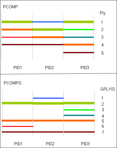
Analysis of Composites

Analysis of composite shells is very similar to the solution of standard shell elements. The primary difference is the use of the PCOMP or PCOMPG property card, instead of PSHELL, to specify shell element properties. From the ply information specified on the PCOMP entry, OptiStruct automatically calculates the effective properties of the shell element.

After the analysis, the available results include shell-type stresses as well as stresses, strains, and failure indices for individual plies and their bonding. These results are controlled by the results flags on the PCOMP or PCOMPG entry and the usual I/O control cards.

PCOMP and PCOMPG define the composite lay-up in two different ways.

PCOMP defines the structure and properties of a composite lay-up which is then assigned to an element. The plies are only defined for that particular property and there is no relationship of plies that reach across several properties.

PCOMPG defines the structure and properties of a composite lay-up allowing for global ply identification which is then assigned to an element. The plies of different PCOMPG definitions can have a relationship because of the use of global ply IDs.

Some remarks are in place regarding the specifics of composite analysis:

Interpretation of Results for Composites

A number of composite-specific results are calculated for composite shell elements. Due to the specialized nature of these results, some explanation is required regarding their meaning.

Classical lamination theory assumes two-dimensional stress-state in individual plies (so-called membrane state). The values of stresses and strains are calculated at the mid-plane of each ply, i.e. halfway between its upper and lower surface. For sufficiently thin plies, these values can be interpreted as representing uniform stress in the ply.

Ply stresses and strains are calculated in coordinate systems aligned with ply material angles as specified on the PCOMP card. In particular, correspond to the primary ply direction, is orthogonal to it, and represents in-plane shear stress.

Ply stresses and strains can also be calculated at planes between the top and bottom planes of each ply. The NDIV field on the CSTRESS and CSTRAIN entries can be used to request the corresponding results for the required planes.

Inter-laminar bonding matrix usually has different material properties and stress-state than the individual plies. The primary stress that is of importance here is inter-laminar shear with two components: and

To facilitate prediction of potential failure of the laminate, failure indices are calculated for plies and bonding material. While there are several theories available for such calculations, their common feature is that failure indices are scaled relative to allowable stresses or strains, so that:

Here, a brief summary of failure theories available is provided.

Hill's Theory of Ply Failure

According to Hill's theory, the ply failure index is calculated as:

Where, X is the allowable stress in the ply material direction (1), Y is the allowable stress in the ply material direction (2), and S is the allowable in-plane shear stress. It should be noted that Hill’s theory does not differentiate between tensile and compressive stresses and it is strongly recommended to use the same values for both allowable stresses, i.e. Xt  = Xc and Yt = Yc. If this suggestion is not adopted, warning messages will be output and the following rules will be applied:  If , X = Xt; otherwise, X = Xc, and similarly for Y and . For the interaction term, if , X = Xt; otherwise, X = Xc.

Hoffman's Theory of Ply Failure

In Hoffman's theory, the ply failure index is calculated as:

Tsai-Wu Theory of Ply Failure

In Tsai-Wu theory, the ply failure index is calculated as:

Where, F12 is a factor to be determined experimentally.

Maximum Strain Theory of Ply Failure

In maximum strain theory, the ply failure index is calculated as the maximum ratio of ply strains to allowable strains:

Where, X is the allowable strain in the ply material direction (1), Y is the allowable strain in the ply material direction (2), and S is the allowable in-plane engineering shear strain. If you provide different values of X and Y for tension and compression, the appropriate values are used depending on the signs of and , respectively. Note that if you set allowable stresses rather than strains on the material data card, the allowable strains are calculated via simple division by the relevant material module.

Bonding Material Failure

The primary failure mode of the bonding material is due to inter-laminar shear. The corresponding failure index is calculated as:

Where, SB is the allowable shear in the bonding material.

Hashin Failure Criteria

The Hashin Failure criteria is calculated for four basic failure modes: in fiber tension, fiber compression, matrix tension, and matrix compression. The corresponding failure indices are calculated as:

Fiber Tension :

Fiber Compression :

Matrix Tension :

Matrix Compression :

Where,

is the allowable homogenized longitudinal tensile strength of the composite.

is the allowable homogenized longitudinal compressive strength of the composite.

is the allowable homogenized transverse tensile strength of the composite.

is the allowable homogenized transverse compressive strength of the fibers.

is the allowable homogenized longitudinal shear strength of the composite.

is the allowable homogenized transverse shear strength of the composite, defined by the Hashin approximation:

is the stress in the 1-direction.

is the stress in the 2-direction.

is the shear stress in 1-2 plane.

Puck Failure Criteria

The Puck Failure Criteria is calculated for two basic failure modes based on 2D plane stress, in fiber failure mode and inter-fiber failure mode. The allowable material data should be specified on the MATF bulk data entry for Puck Failure Criterion. The corresponding failure indices are calculated as:

Fiber Failure Mode

Fiber Tension :

Fiber Compression :

Inter-Fiber Failure Mode

Mode A :

Mode B :

Mode C :

Where,

is the allowable longitudinal tensile strength.

is the allowable longitudinal compressive strength.

is the allowable transverse tensile strength.

is the allowable transverse compressive strength.

is the allowable shear strength.

is the stress in the 1-direction.

is the stress in the 2-direction.

is the shear stress in 1-2 plane.

is the failure envelope factor 12 (+).

is the failure envelope factor 12 (-).

is the failure envelope factor 22 (-).

Final Failure Index for Composite Element

After calculation of failure indices for individual plies, the potential failure index for the composite shell element is obtained. This is based on the premise that failure of a single layer qualifies as failure of the composite. Thus, the failure index for composite element is calculated as the maximum of all computed ply and bonding failure indices (note that only plies with requested stress output are taken into account here).

Comparison of laminate modeled with PCOMP and PCOMPG